Solver#
The rateslib.solver module includes a Solver class
which iteratively solves for the parameters of Curve objects, to
fit the given market data of calibrating Instruments.
This module relies on the utility module dual for gradient based optimization.
|
A numerical solver to determine node values on multiple curves simultaneously. |
Parameters#
The Solver solves the following least squares
objective function:
where \(\mathbf{S}\) are the known calibrating instrument rates, \(\mathbf{r}\) are the determined instrument rates based on the solved parameters, \(\mathbf{v}\), and \(\mathbf{W}\) is a diagonal matrix of weights.
Each curve type has the following parameters:
Parameter |
Type |
Summary |
Affected by |
|---|---|---|---|
|
Hyper parameter |
Equation or mechanism to determine intermediate values not defined explicitly
by |
No |
|
Hyper parameters |
Fixed points which implicitly impact the interpolated values across the curve. |
No |
|
Hyper parameters |
Framework for defining the (log) cubic spline structure which implicitly impacts the interpolated values across the curve. |
No |
|
Hyper parameters |
Method used to control spline curves on the left and right boundaries. |
No |
|
Parameters |
The explicit values associated with node dates. |
Calibrating Curves#
Thus, in order to calibrate or solve curves the hyper parameters must already
be defined, so that nodes, interpolation, t and endpoints must all
be configured. These will not be changed by the Solver.
The nodes values (the parameters) should be initialised with sensible values
from which the
optimizer will start. However, it is usually quite robust and should be able to solve
from a variety of initialised node values.
We define a simple Curve using default hyper parameters
and only a few nodes.
In [1]: ll_curve = Curve(
   ...:     nodes={
   ...:         dt(2022,1,1): 1.0,
   ...:         dt(2023,1,1): 0.99,
   ...:         dt(2024,1,1): 0.979,
   ...:         dt(2025,1,3): 0.967
   ...:     },
   ...:     id="curve",
   ...: )
   ...:
Next, we must define the instruments which will instruct the solution.
In [2]: instruments = [
   ...:     IRS(dt(2022, 1, 1), "1Y", "A", curves="curve"),
   ...:     IRS(dt(2022, 1, 1), "2Y", "A", curves="curve"),
   ...:     IRS(dt(2022, 1, 1), "3Y", "A", curves="curve"),
   ...: ]
   ...:
There are a number of different mechanisms for the way in which this can be done, but the example here reflects best practice as demonstrated in pricing mechanisms.
Once a suitable, and valid, set of instruments has been configured we can supply it,
and the curves, to the solver. We must also supply some target rates, s, and
the optimizer will update the curves.
In [3]: solver = Solver(
...: curves = [ll_curve],
...: instruments = instruments,
...: s = [1.0, 1.6, 2.0],
...: )
...:
SUCCESS: `func_tol` reached after 4 iterations (levenberg_marquardt), `f_val`: 9.549288083712273e-14, `time`: 0.0057s
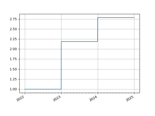
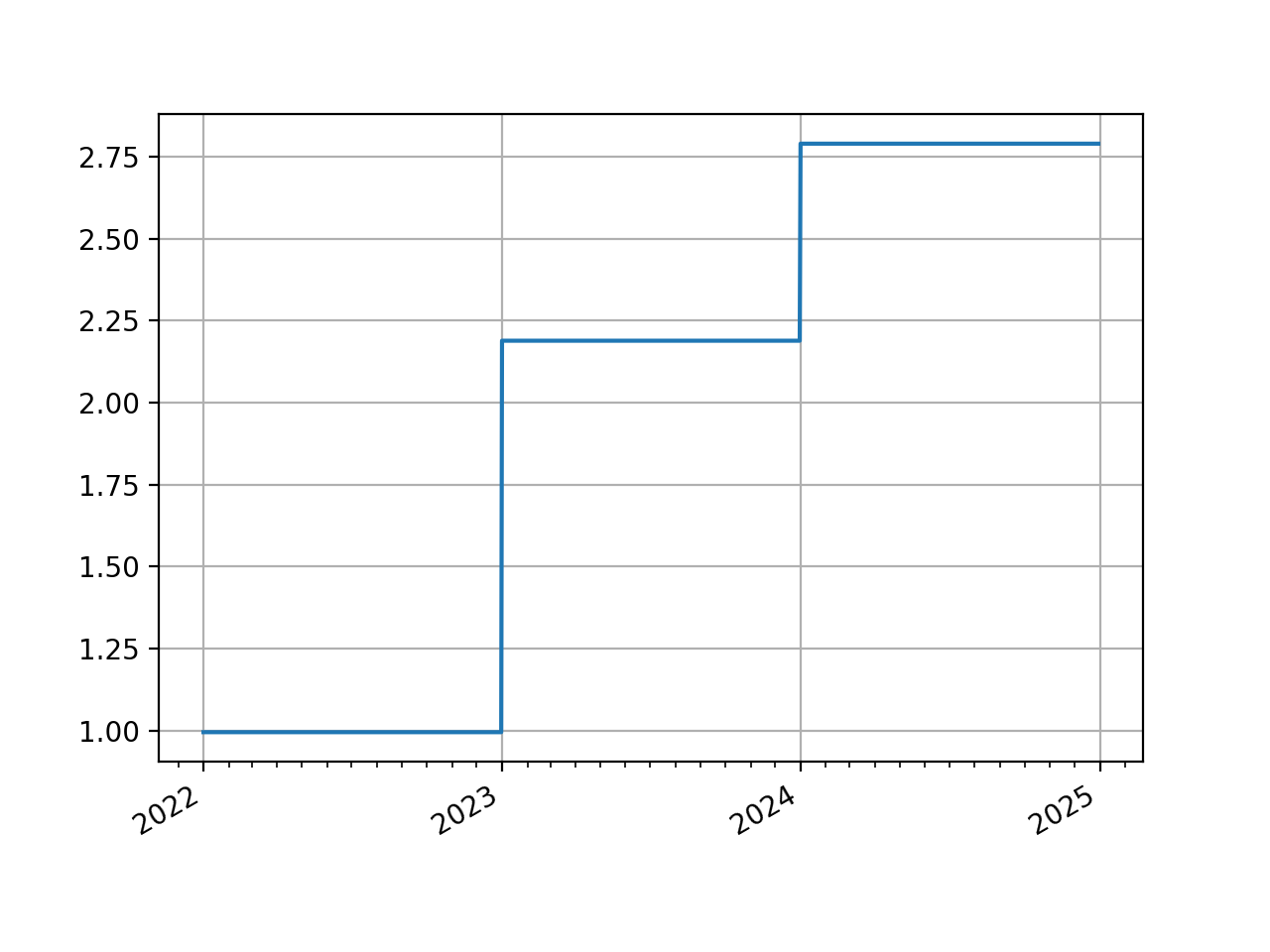
In [4]: ll_curve.plot("1D")
Out[4]:
(<Figure size 640x480 with 1 Axes>,
<Axes: >,
[<matplotlib.lines.Line2D at 0x7f0a9fadff90>])
(Source code, png, hires.png, pdf)

The values of the solver.s can be updated and the curves can be redetermined
In [5]: print(instruments[1].rate(ll_curve).real)
1.5999999997080336

In [6]: solver.s[1] = 1.5

In [7]: solver.iterate()
SUCCESS: `func_tol` reached after 3 iterations (levenberg_marquardt), `f_val`: 1.6299982557749375e-12, `time`: 0.0097s

In [8]: print(instruments[1].rate(ll_curve).real)
1.500001236890998
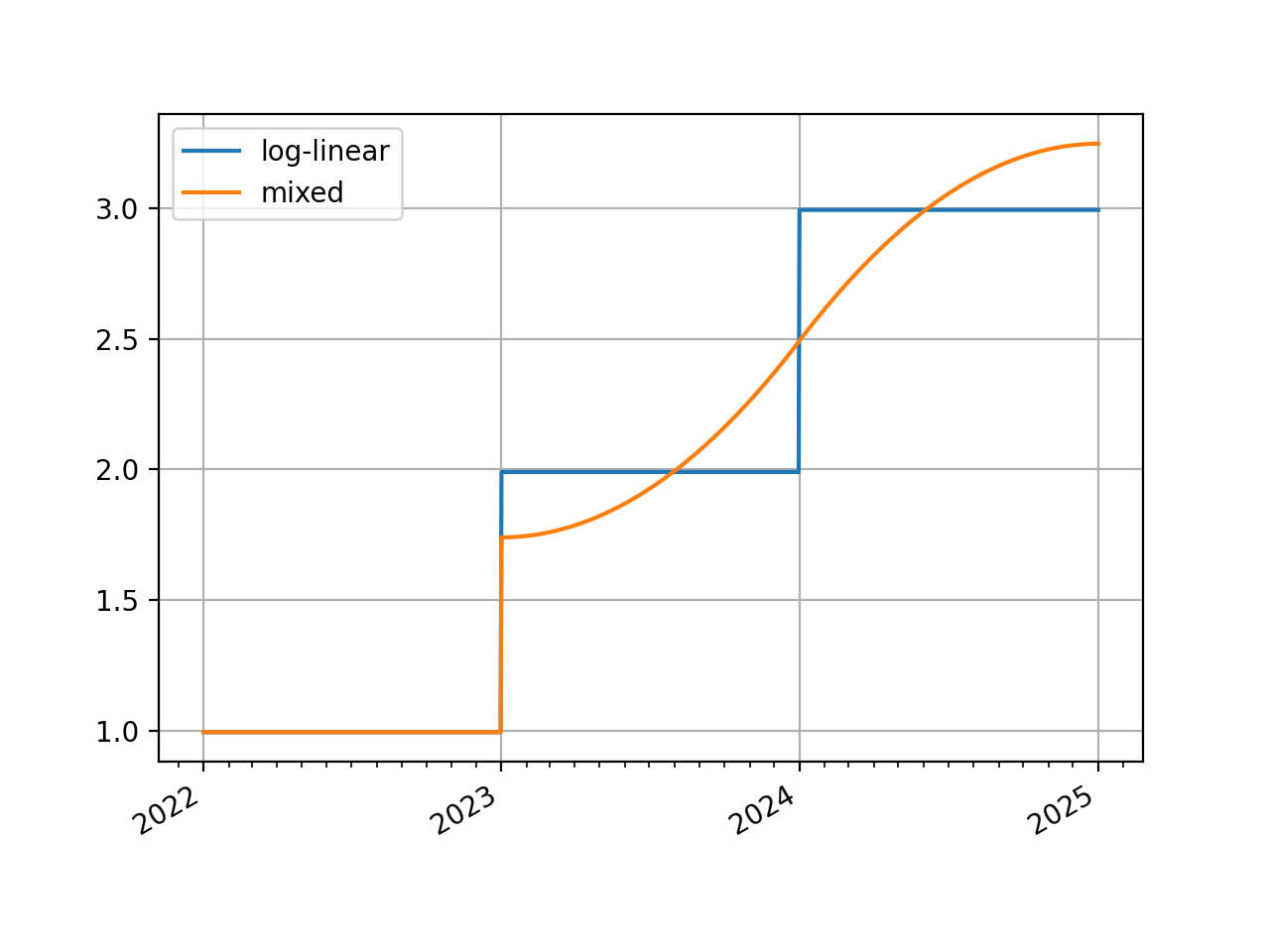
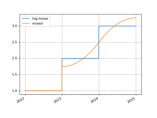
Changing the hyper parameters of a curve does not require any fundamental
change to the input arguments to the Solver.
Here a mixed interpolation scheme is used and the Curve
calibrated.
In [9]: mixed_curve = Curve(
   ...:     nodes={
   ...:         dt(2022,1,1): 1.0,
   ...:         dt(2023,1,1): 0.99,
   ...:         dt(2024,1,1): 0.965,
   ...:         dt(2025,1,3): 0.93,
   ...:     },
   ...:     interpolation="log_linear",
   ...:     t = [dt(2023,1,1), dt(2023,1,1), dt(2023,1,1), dt(2023,1,1), dt(2024,1,1), dt(2025,1,3), dt(2025,1,3), dt(2025,1,3), dt(2025,1,3)],
   ...:     id="curve",
   ...: )
   ...:

In [10]: solver = Solver(
   ....:     curves = [mixed_curve],
   ....:     instruments = instruments,
   ....:     s = [1.0, 1.5, 2.0],
   ....: )
   ....:
SUCCESS: `func_tol` reached after 4 iterations (levenberg_marquardt), `f_val`: 2.0488787156020367e-14, `time`: 0.0058s

In [11]: ll_curve.plot("1D", comparators=[mixed_curve], labels=["log-linear", "mixed"])
Out[11]:
(<Figure size 640x480 with 1 Axes>,
 <Axes: >,
 [<matplotlib.lines.Line2D at 0x7f0a9fab4890>,
  <matplotlib.lines.Line2D at 0x7f0a9f8ed290>])
(Source code, png, hires.png, pdf)
Algorithms#
In the defaults settings of rateslib, Solver uses
a “levenberg_marquardt” algorithm.
There is an option to use a “gauss_newton” algorithm which is faster if the initial guess is reasonable. This should be used where possible, but this is a more unstable algorithm so is not set as the default.
For other debugging procedures the “gradient_descent” method is available although this is not recommended due to computational inefficiency.
Details on these algorithms are provided in the rateslib
supplementary materials.
Weights#
The argument weights allows certain instrument rates to be targeted with
greater priority than others. In the above examples this was of no relevance since
in all previous cases the minimum solution of zero was fully attainable.
The following pathological example, where the same instruments are provided multiple times with different rates, shows the effect.
In [12]: instruments = [
   ....:     IRS(dt(2022, 1, 1), "1Y", "A", curves="curve"),
   ....:     IRS(dt(2022, 1, 1), "2Y", "A", curves="curve"),
   ....:     IRS(dt(2022, 1, 1), "3Y", "A", curves="curve"),
   ....:     IRS(dt(2022, 1, 1), "1Y", "A", curves="curve"),
   ....:     IRS(dt(2022, 1, 1), "2Y", "A", curves="curve"),
   ....:     IRS(dt(2022, 1, 1), "3Y", "A", curves="curve"),
   ....: ]
   ....:

In [13]: solver = Solver(
   ....:     curves = [mixed_curve],
   ....:     instruments = instruments,
   ....:     s = [1.0, 1.1, 1.2, 5.0, 5.1, 5.2],
   ....:     weights = [1, 1, 1, 1e-4, 1e-4, 1e-4],
   ....: )
   ....:
SUCCESS: `conv_tol` reached after 7 iterations (levenberg_marquardt), `f_val`: 0.0047995200479952005, `time`: 0.0165s

In [14]: for instrument in instruments:
   ....:     print(float(instrument.rate(solver=solver)))
   ....:
1.0003999600039903
1.1003999600039887
1.200399960003984
1.0003999600039903
1.1003999600039887
1.200399960003984

In [15]: solver = Solver(
   ....:     curves = [mixed_curve],
   ....:     instruments = instruments,
   ....:     s = [1.0, 1.1, 1.2, 5.0, 5.1, 5.2],
   ....:     weights = [1e-4, 1e-4, 1e-4, 1, 1, 1],
   ....: )
   ....:
FAILURE: `max_iter` breached after 100 iterations (levenberg_marquardt), `f_val`: 0.0047995200479952005, `time`: 0.2082s

In [16]: for instrument in instruments:
   ....:     print(float(instrument.rate(solver=solver)))
   ....:
4.999600039996006
5.099600039996002
5.199600039996004
4.999600039996006
5.099600039996002
5.199600039996004
Dependency Chains#
In real fixed income trading environments every curve should be synchronous and
dependencies should use the same construction method in one division as in another.
The pre_solvers argument allows a chain of Solver s.
Here a SOFR curve is constructed via a solver and is then added to another solver
which solves an ESTR curve. There is no technical dependence here of one on the
other so these solvers could be arranged in either order.
In [17]: sofr_curve = Curve(
   ....:     nodes={
   ....:         dt(2022, 1, 1): 1.0,
   ....:         dt(2023, 1, 1): 1.0,
   ....:         dt(2024, 1, 1): 1.0,
   ....:         dt(2025, 1, 1): 1.0,
   ....:     },
   ....:     id="sofr",
   ....: )
   ....:

In [18]: sofr_instruments = [
   ....:     IRS(dt(2022, 1, 1), "1Y", "A", currency="usd", curves="sofr"),
   ....:     IRS(dt(2022, 1, 1), "2Y", "A", currency="usd", curves="sofr"),
   ....:     IRS(dt(2022, 1, 1), "3Y", "A", currency="usd", curves="sofr"),
   ....: ]
   ....:

In [19]: sofr_solver = Solver(
   ....:     curves = [sofr_curve],
   ....:     instruments = sofr_instruments,
   ....:     s = [2.5, 3.0, 3.5],
   ....: )
   ....:
SUCCESS: `func_tol` reached after 4 iterations (levenberg_marquardt), `f_val`: 4.659124754473029e-13, `time`: 0.0056s

In [20]: estr_curve = Curve(
   ....:     nodes={
   ....:         dt(2022, 1, 1): 1.0,
   ....:         dt(2023, 1, 1): 1.0,
   ....:         dt(2024, 1, 1): 1.0,
   ....:         dt(2025, 1, 1): 1.0,
   ....:     },
   ....:     id="estr",
   ....: )
   ....:

In [21]: estr_instruments = [
   ....:     IRS(dt(2022, 1, 1), "1Y", "A", currency="eur", curves="estr"),
   ....:     IRS(dt(2022, 1, 1), "2Y", "A", currency="eur", curves="estr"),
   ....:     IRS(dt(2022, 1, 1), "3Y", "A", currency="eur", curves="estr"),
   ....: ]
   ....:

In [22]: estr_solver = Solver(
   ....:     curves = [estr_curve],
   ....:     instruments = estr_instruments,
   ....:     s = [1.25, 1.5, 1.75],
   ....:     pre_solvers=[sofr_solver]
   ....: )
   ....:
SUCCESS: `func_tol` reached after 4 iterations (levenberg_marquardt), `f_val`: 3.1986237566494413e-13, `time`: 0.0055s
It is possible to create only a single solver using the two curves and six instruments above. However, in practice it is less efficient to solve independent solvers within the same framework. And practically, this is not usually how trading teams are configured, all as one big group. Normally siloed teams are responsible for their own subsections, be it one currency or another, or different product types.
Multi-Currency Instruments#
Multi-currency derivatives rely on FXForwards. In this
example we establish a new cash-collateral discount curve and use
XCS within a Solver.
In [23]: eurusd = Curve(
....: nodes={
....: dt(2022, 1, 1): 1.0,
....: dt(2023, 1, 1): 1.0,
....: dt(2024, 1, 1): 1.0,
....: dt(2025, 1, 1): 1.0,
....: },
....: id="eurusd",
....: )
....:
In [24]: fxr = FXRates({"eurusd": 1.10}, settlement=dt(2022, 1, 3))
In [25]: fxf = FXForwards(
....: fx_rates=fxr,
....: fx_curves={
....: "eureur": estr_curve,
....: "eurusd": eurusd,
....: "usdusd": sofr_curve,
....: }
....: )
....:
In [26]: kwargs={
....: "currency": "eur",
....: "leg2_currency": "usd",
....: "curves": ["estr", "eurusd", "sofr", "sofr"],
....: }
....:
In [27]: xcs_instruments = [
....: XCS(dt(2022, 1, 1), "1Y", "A", **kwargs),
....: XCS(dt(2022, 1, 1), "2Y", "A", **kwargs),
....: XCS(dt(2022, 1, 1), "3Y", "A", **kwargs),
....: ]
....:
In [28]: xcs_solver = Solver(
....: curves = [eurusd],
....: instruments = xcs_instruments,
....: s = [-10, -15, -20],
....: fx=fxf,
....: pre_solvers=[estr_solver],
....: )
....:
SUCCESS: `func_tol` reached after 3 iterations (levenberg_marquardt), `f_val`: 3.0042493839090535e-17, `time`: 0.0327s
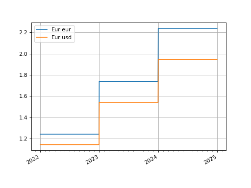
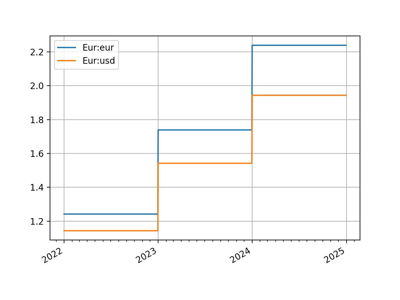
In [29]: estr_curve.plot("1d", comparators=[eurusd], labels=["Eur:eur", "Eur:usd"])
Out[29]:
(<Figure size 640x480 with 1 Axes>,
<Axes: >,
[<matplotlib.lines.Line2D at 0x7f0a9f7dbc50>,
<matplotlib.lines.Line2D at 0x7f0a9f774450>])
(Source code, png, hires.png, pdf)

Calibration Instrument Error#
Depending upon the hyper parameters, parameters and calibrating instrument choices, the optimized solution may well lead to curves that do not completely reprice the calibrating instruments. Sometimes this is representative of errors in the construction process, and at other times this is completely desirable.
When the Solver is initialised and iterates it will print
an output to console indicating a success or failure and the value of the
objective function. If this value is very small, that already indicates that there is
no error in any instruments. However for cases where the curve is over-specified, error
is to be expected.
In [30]: solver_with_error = Solver(
   ....:     curves=[
   ....:         Curve(
   ....:             nodes={dt(2022, 1, 1): 1.0, dt(2022, 7, 1): 1.0, dt(2023, 1, 1): 1.0},
   ....:             id="curve1"
   ....:         )
   ....:     ],
   ....:     instruments=[
   ....:         IRS(dt(2022, 1, 1), "1M", "A", curves="curve1"),
   ....:         IRS(dt(2022, 1, 1), "2M", "A", curves="curve1"),
   ....:         IRS(dt(2022, 1, 1), "3M", "A", curves="curve1"),
   ....:         IRS(dt(2022, 1, 1), "4M", "A", curves="curve1"),
   ....:         IRS(dt(2022, 1, 1), "8M", "A", curves="curve1"),
   ....:         IRS(dt(2022, 1, 1), "12M", "A", curves="curve1"),
   ....:     ],
   ....:     s=[2.0, 2.2, 2.3, 2.4, 2.45, 2.55],
   ....:     instrument_labels=["1m", "2m", "3m", "4m", "8m", "12m"],
   ....: )
   ....:
SUCCESS: `conv_tol` reached after 4 iterations (levenberg_marquardt), `f_val`: 0.08763280492897038, `time`: 0.0062s

In [31]: solver_with_error.error
Out[31]:
e77b7_  1m     22.80
        2m      2.99
        3m     -6.79
        4m    -16.59
        8m     -4.59
        12m     2.30
dtype: float64
Composite, Proxy and Multi-CSA Curves#
CompositeCurve, ProxyCurve and
MultiCsaCurve do not
have their own parameters. These rely on the parameters from other fundamental curves.
It is possible to create a Solver defined with Instruments that reference these
complex curves as pricing curves with the Solver updating the underlying
parameters of the fundamental curves.
This does not require much additional configuration, it simply requires ensuring all necessary curves are documented.
Below we will calculate a EUR IRS defined by a CompositeCurve and a Curve,
a USD IRS defined just by a Curve, and then create an FXForwards
defined with USD collateral, but calibrate a solver by
XCS instruments priced with EUR collateral.
In [32]: eureur = Curve({dt(2022, 1, 1): 1.0, dt(2023, 1, 1): 1.0}, id="eureur")

In [33]: eurspd = Curve({dt(2022, 1, 1): 1.0, dt(2023, 1, 1): 0.999}, id="eurspd")

In [34]: eur3m = CompositeCurve([eureur, eurspd], id="eur3m")

In [35]: usdusd = Curve({dt(2022, 1, 1): 1.0, dt(2023, 1, 1): 1.0}, id="usdusd")

In [36]: eurusd = Curve({dt(2022, 1, 1): 1.0, dt(2023, 1, 1): 1.0}, id="eurusd")

In [37]: fxr = FXRates({"eurusd": 1.1}, settlement=dt(2022, 1, 3))

In [38]: fxf = FXForwards(
   ....:     fx_rates=fxr,
   ....:     fx_curves={
   ....:         "eureur": eureur,
   ....:         "usdusd": usdusd,
   ....:         "eurusd": eurusd,
   ....:     }
   ....: )
   ....:

In [39]: usdeur = fxf.curve("usd", "eur", id="usdeur")

In [40]: instruments = [
   ....:     IRS(dt(2022, 1, 1), "1Y", "A", currency="eur", curves=["eur3m", "eureur"]),
   ....:     IRS(dt(2022, 1, 1), "1Y", "A", currency="usd", curves="usdusd"),
   ....:     XCS(dt(2022, 1, 1), "1Y", "A", currency="eur", leg2_currency="usd", curves=["eureur", "eureur", "usdusd", "usdeur"]),
   ....: ]
   ....:

In [41]: solver = Solver(curves=[eureur, eur3m, usdusd, eurusd, usdeur], instruments=instruments, s=[2.0, 2.7, -15], fx=fxf)
SUCCESS: `func_tol` reached after 3 iterations (levenberg_marquardt), `f_val`: 3.73941410218606e-12, `time`: 0.0124s
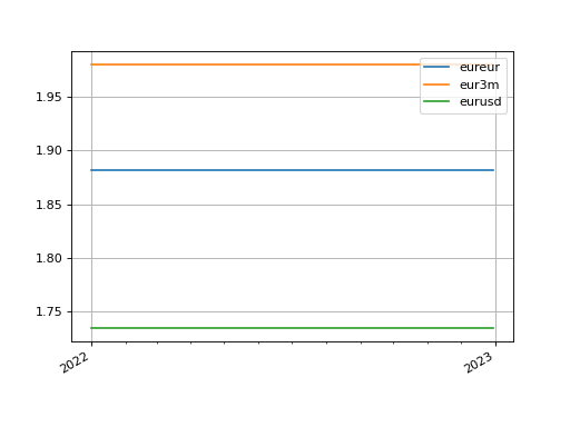
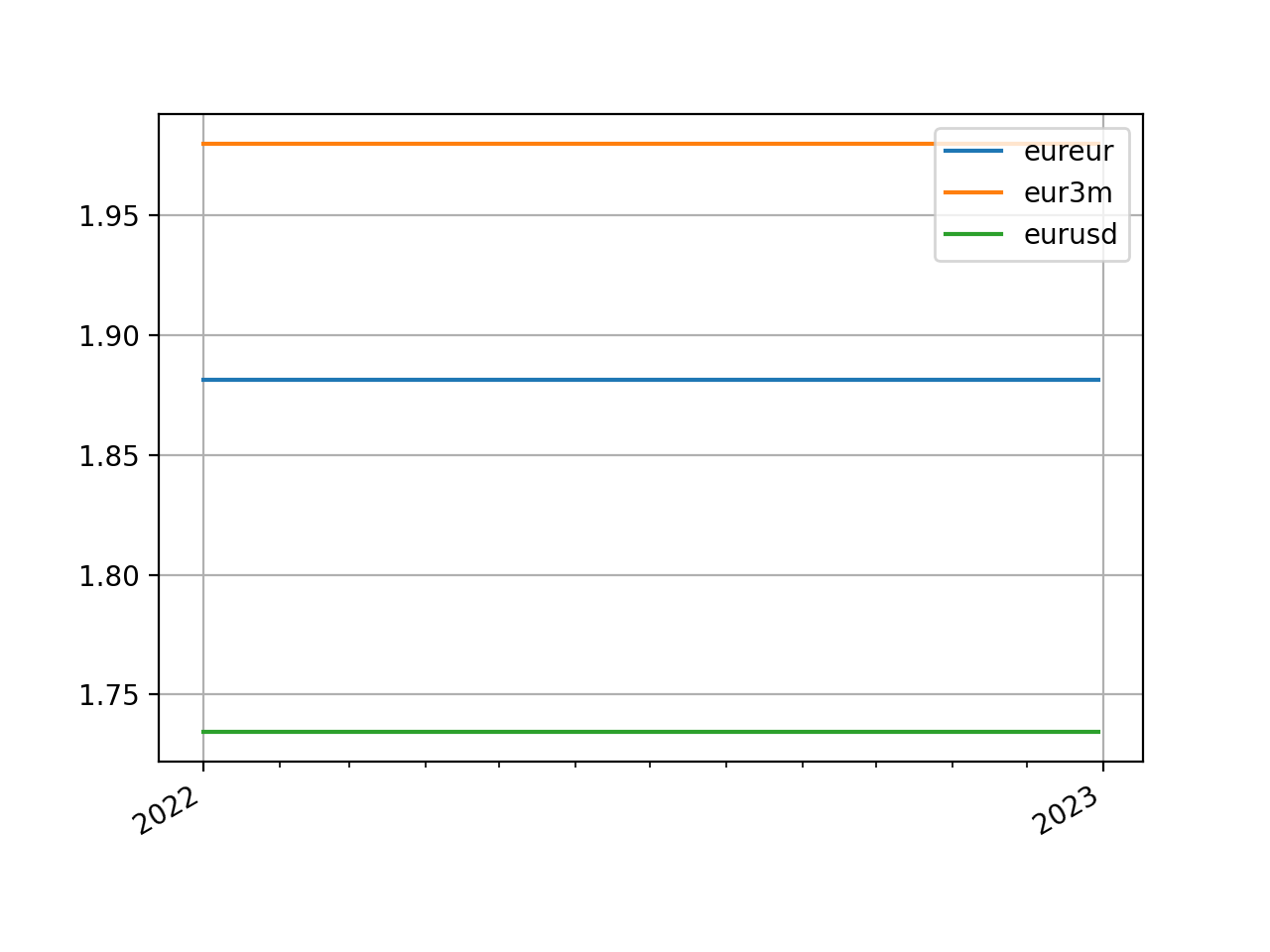
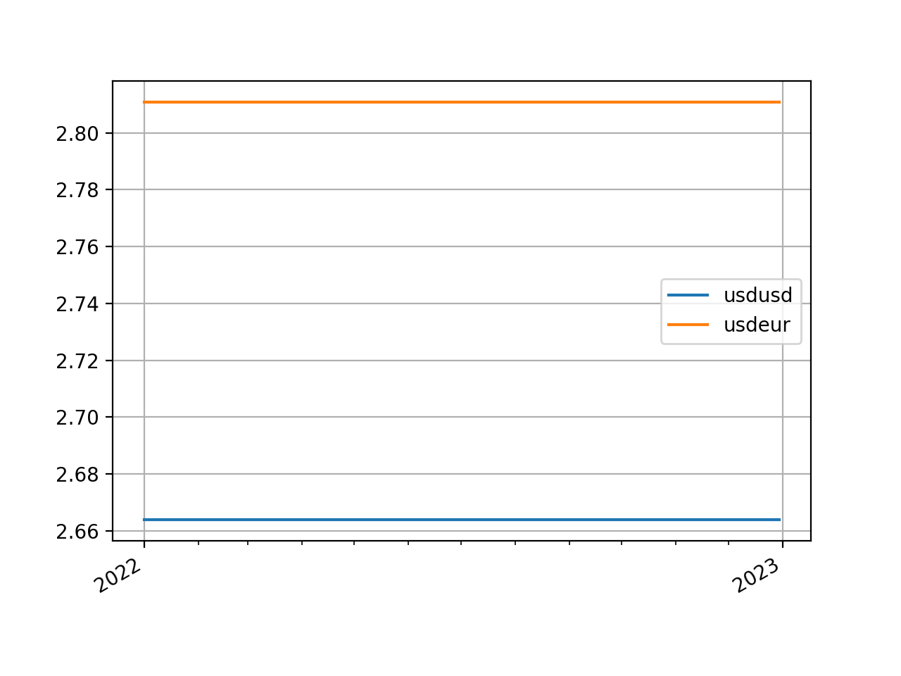
We can plot all five curves defined above by the 3 fundamental curves, ‘eureur’, ‘usdusd’, ‘eurusd’.
In [42]: eureur.plot("1d", comparators=[eur3m, eurusd], labels=["eureur", "eur3m", "eurusd"])
Out[42]:
(<Figure size 640x480 with 1 Axes>,
 <Axes: >,
 [<matplotlib.lines.Line2D at 0x7f0a9f593c50>,
  <matplotlib.lines.Line2D at 0x7f0a9f3e3050>,
  <matplotlib.lines.Line2D at 0x7f0a9f3e3950>])

In [43]: usdusd.plot("1d", comparators=[usdeur], labels=["usdusd", "usdeur"])
Out[43]:
(<Figure size 640x480 with 1 Axes>,
 <Axes: >,
 [<matplotlib.lines.Line2D at 0x7f0a9f98a9d0>,
  <matplotlib.lines.Line2D at 0x7f0a9f443c90>])
(Source code, png, hires.png, pdf)

(Source code, png, hires.png, pdf)
