Replicating a SOFR Curve & Swap from Bloomberg’s SWPM#
At a point in time on Thu 17th Aug 2023 loading the SWPM function in Bloomberg presented the following default SOFR curve data:
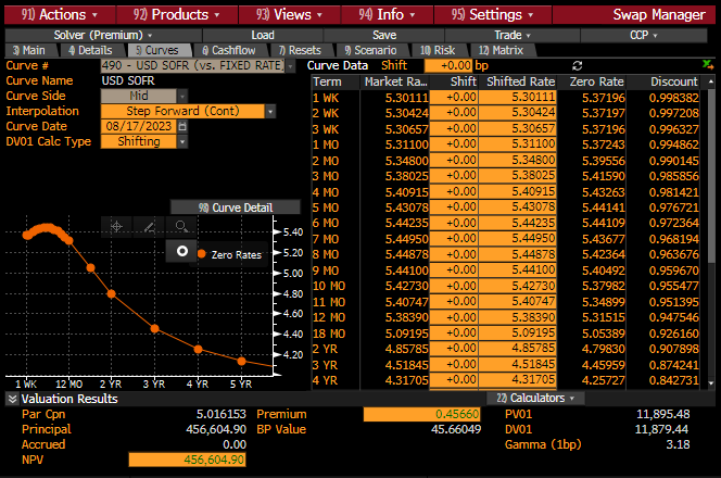
We can replicate the input data for the Curve in a table as follows:
In [1]: data = DataFrame({
   ...:     "Term": ["1W", "2W", "3W", "1M", "2M", "3M", "4M", "5M", "6M", "7M", "8M", "9M", "10M", "11M", "12M", "18M", "2Y", "3Y", "4Y"],
   ...:     "Rate": [5.30111, 5.30424, 5.30657, 5.31100, 5.34800, 5.38025, 5.40915, 5.43078, 5.44235, 5.44950, 5.44878, 5.44100, 5.42730, 5.40747, 5.3839, 5.09195, 4.85785, 4.51845, 4.31705],
   ...: })
   ...:

In [2]: data["Termination"] = [add_tenor(dt(2023, 8, 21), _, "F", "nyc") for _ in data["Term"]]

In [3]: with option_context("display.float_format", lambda x: '%.6f' % x):
   ...:     print(data)
   ...:
   Term     Rate Termination
0    1W 5.301110  2023-08-28
1    2W 5.304240  2023-09-05
2    3W 5.306570  2023-09-11
3    1M 5.311000  2023-09-21
4    2M 5.348000  2023-10-23
5    3M 5.380250  2023-11-21
6    4M 5.409150  2023-12-21
7    5M 5.430780  2024-01-22
8    6M 5.442350  2024-02-21
9    7M 5.449500  2024-03-21
10   8M 5.448780  2024-04-22
11   9M 5.441000  2024-05-21
12  10M 5.427300  2024-06-21
13  11M 5.407470  2024-07-22
14  12M 5.383900  2024-08-21
15  18M 5.091950  2025-02-21
16   2Y 4.857850  2025-08-21
17   3Y 4.518450  2026-08-21
18   4Y 4.317050  2027-08-23
Bloomberg defaults to a “Step Forward (cont)” interpolation mode, this is effectively the
same as “log_linear” in rateslib’s formulation for Curves. We will configure DF
nodes dates to be on the termination date of the swaps:
In [4]: sofr = Curve(
   ...:     id="sofr",
   ...:     convention="Act360",
   ...:     calendar="nyc",
   ...:     modifier="MF",
   ...:     interpolation="log_linear",
   ...:     nodes={
   ...:         **{dt(2023, 8, 17): 1.0},  # <- this is today's DF,
   ...:         **{_: 1.0 for _ in data["Termination"]},
   ...:     }
   ...: )
   ...:
Now we will calibrate the curve to the given swap market prices, using a global
Solver, passing in the calibrating instruments and rates.
In [5]: sofr_args = dict(effective=dt(2023, 8, 21), spec="usd_irs", curves="sofr")

In [6]: solver = Solver(
   ...:     curves=[sofr],
   ...:     instruments=[IRS(termination=_, **sofr_args) for _ in data["Termination"]],
   ...:     s=data["Rate"],
   ...:     instrument_labels=data["Term"],
   ...:     id="us_rates",
   ...: )
   ...:
SUCCESS: `func_tol` reached after 5 iterations (levenberg_marquardt), `f_val`: 3.116743265440467e-17, `time`: 0.0562s

In [7]: data["DF"] = [float(sofr[_]) for _ in data["Termination"]]

In [8]: with option_context("display.float_format", lambda x: '%.6f' % x):
   ...:     print(data)
   ...:
   Term     Rate Termination       DF
0    1W 5.301110  2023-08-28 0.998382
1    2W 5.304240  2023-09-05 0.997208
2    3W 5.306570  2023-09-11 0.996327
3    1M 5.311000  2023-09-21 0.994862
4    2M 5.348000  2023-10-23 0.990145
5    3M 5.380250  2023-11-21 0.985856
6    4M 5.409150  2023-12-21 0.981421
7    5M 5.430780  2024-01-22 0.976721
8    6M 5.442350  2024-02-21 0.972364
9    7M 5.449500  2024-03-21 0.968194
10   8M 5.448780  2024-04-22 0.963676
11   9M 5.441000  2024-05-21 0.959670
12  10M 5.427300  2024-06-21 0.955477
13  11M 5.407470  2024-07-22 0.951395
14  12M 5.383900  2024-08-21 0.947546
15  18M 5.091950  2025-02-21 0.926160
16   2Y 4.857850  2025-08-21 0.907898
17   3Y 4.518450  2026-08-21 0.874241
18   4Y 4.317050  2027-08-23 0.842731
Notice that the DFs are the same as those in SWPM (at least to a visible 1e-6 tolerance).
Next we will create a swap in SWPM and also create the same swap in rateslib. The metrics that SWPM and rateslib generate for npv, delta (DV01), gamma and analytic delta (PV01) are the same to within a very small tolerance.
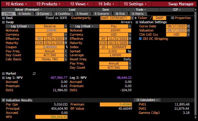
In [9]: irs = IRS(
   ...:     effective=dt(2023, 11, 21),
   ...:     termination=dt(2025, 2, 21),
   ...:     notional=-100e6,
   ...:     fixed_rate=5.40,
   ...:     curves="sofr",
   ...:     spec="usd_irs",
   ...: )
   ...:

In [10]: irs.npv(solver=solver)
Out[10]: <Dual: 456622.098604, (sofr0, sofr1, sofr2, ...), [0.0, 0.0, 0.0, ...]>

In [11]: irs.delta(solver=solver).sum()
Out[11]:
local_ccy  display_ccy
usd        usd           -11879.94
dtype: float64

In [12]: irs.gamma(solver=solver).sum().sum()
Out[12]: 3.176665278863451

In [13]: irs.analytic_delta(curve=sofr)
Out[13]: <Dual: -11896.008577, (sofr0, sofr1, sofr2, ...), [-0.0, -0.0, -0.0, ...]>
Finally we can double check the cashflows and cashflows_table of the swap.
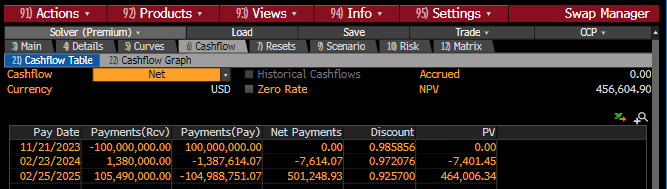
In [14]: irs.cashflows_table(solver=solver)
Out[14]:
local_ccy            USD
collateral_ccy       NaN
payment
2024-02-23      -7613.74
2025-02-25     501239.07

In [15]: irs.cashflows(solver=solver)
Out[15]:
               Type   Period  Ccy  Acc Start    Acc End    Payment Convention  DCF      Notional   DF Collateral  Rate  Spread    Cashflow         NPV  FX Rate     NPV Ccy
leg1 0  FixedPeriod     Stub  USD 2023-11-21 2024-02-21 2024-02-23     act360 0.26 -100000000.00 0.97       None  5.40     NaN  1380000.00  1341464.35     1.00  1341464.35
     1  FixedPeriod  Regular  USD 2024-02-21 2025-02-21 2025-02-25     act360 1.02 -100000000.00 0.93       None  5.40     NaN  5490000.00  5082380.28     1.00  5082380.28
leg2 0  FloatPeriod     Stub  USD 2023-11-21 2024-02-21 2024-02-23     act360 0.26  100000000.00 0.97       None  5.43    0.00 -1387613.74 -1348865.48     1.00 -1348865.48
     1  FloatPeriod  Regular  USD 2024-02-21 2025-02-21 2025-02-25     act360 1.02  100000000.00 0.93       None  4.91    0.00 -4988760.93 -4618357.05     1.00 -4618357.05