LineCurve

class rateslib.curves.LineCurve(*args, **kwargs)

Bases: Curve

Curve based on value parametrisation at given node dates with interpolation.

Parameters:

• nodes (dict[datetime: float]) – Parameters of the curve denoted by a node date and a corresponding value at that point.

• interpolation (str in {"log_linear", "linear"} or callable) – The interpolation used in the non-spline section of the curve. That is the part of the curve between the first node in nodes and the first knot in t. If a callable, this allows a user-defined interpolation scheme, and this must have the signature method(date, nodes), where date is the datetime whose DF will be returned and nodes is as above and is passed to the callable.

• t (list[datetime], optional) – The knot locations for the B-spline cubic interpolation section of the curve. If None all interpolation will be done by the method specified in interpolation.

• c (list[float], optional) – The B-spline coefficients used to define the log-cubic spline. If not given, which is the expected case, uses csolve() to calculate these automatically.

• endpoints (str or list, optional) – The left and right endpoint constraint for the spline solution. Valid values are in {“natural”, “not_a_knot”}. If a list, supply the left endpoint then the right endpoint.

• id (str, optional, set by Default) – The unique identifier to distinguish between curves in a multi-curve framework.

• convention (str, optional,) – This argument is not used by LineCurve. It is included for signature consistency with Curve.

• modifier (str, optional) – This argument is not used by LineCurve. It is included for signature consistency with Curve.

• calendar (calendar or str, optional) – This argument is not used by LineCurve. It is included for signature consistency with Curve.

• ad (int in {0, 1, 2}, optional) – Sets the automatic differentiation order. Defines whether to convert node values to float, Dual or Dual2. It is advised against using this setting directly. It is mainly used internally.

Notes

This curve type is value based and it is parametrised by a set of (date, value) pairs set as nodes. The initial node date of the curve is defined to be today, and can take a general value. The initial value will be affected by a Solver.

Note

This curve type can only ever be used for forecasting rates and projecting cashflow calculations. It cannot be used to discount cashflows becuase it is not DF based and there is no mathematical one-to-one conversion available to imply DFs.

Intermediate values are determined through interpolation. If local interpolation is adopted a value for an arbitrary date is dependent only on its immediately neighbouring nodes via the interpolation routine. Available options are:

• “linear” (default for this curve type)

• “log_linear” (useful for values that exponential, e.g. stock indexes or GDP)

• “flat_forward”, (useful for replicating a DF based log-linear type curve)

• “flat_backward”,

And also the following which are not recommended for this curve type:

• “linear_index”

• “linear_zero_rate”,

Global interpolation in the form of a cubic spline is also configurable with the parameters t, c and endpoints. See splines for instruction of knot sequence calibration. Values before the first knot in t will be determined through the local interpolation method.

This curve type cannot return arbitrary tenor rates. It will only return a single value which is applicable to that date. It is recommended to review RFR and IBOR Indexing to ensure indexing is done in a way that is consistent with internal instrument configuration.

Examples

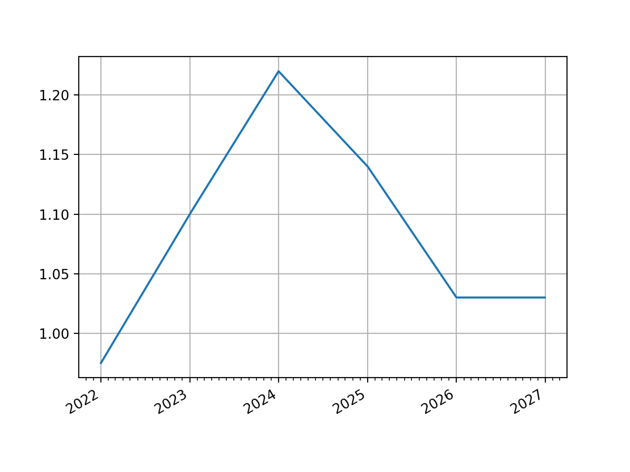
In [1]: line_curve = LineCurve(
   ...:     nodes={
   ...:         dt(2022,1,1): 0.975,  # <- initial value is general
   ...:         dt(2023,1,1): 1.10,
   ...:         dt(2024,1,1): 1.22,
   ...:         dt(2025,1,1): 1.14,
   ...:         dt(2026,1,1): 1.03,
   ...:         dt(2027,1,1): 1.03,
   ...:     },
   ...:     interpolation="linear",
   ...: )
   ...: 

In [2]: line_curve.plot("1d")
Out[2]: 
(<Figure size 640x480 with 1 Axes>,
 <Axes: >,
 [<matplotlib.lines.Line2D at 0x7f0aa51457d0>])

(Source code, png, hires.png, pdf)

Attributes Summary

collateral

Methods Summary

copy()	Create an identical copy of the curve object.
csolve()	Solves and sets the coefficients, c, of the PPSpline.
from_json(curve, **kwargs)	Reconstitute a curve from JSON.
plot(tenor[, right, left, comparators, ...])	Plot given forward tenor rates from the curve.
rate(effective, *args)	Return the curve value for a given date.
roll(tenor)	Create a new curve with its shape translated in time
shift(spread[, id, composite, collateral])	Raise or lower the curve in parallel by a set number of basis points.
to_json()	Convert the parameters of the curve to JSON format.
translate(start[, t])	Create a new curve with an initial node date moved forward keeping all else constant.

Attributes Documentation

collateral = None

Methods Documentation

copy()

Create an identical copy of the curve object.

Return type:

Curve or LineCurve

csolve()

Solves and sets the coefficients, c, of the PPSpline.

Return type:

None

Notes

Only impacts curves which have a knot sequence, t, and a PPSpline. Only solves if c not given at curve initialisation.

Uses the spline_endpoints attribute on the class to determine the solving method.

classmethod from_json(curve, **kwargs)

Reconstitute a curve from JSON.

Parameters:

curve (str) – The JSON string representation of the curve.

Return type:

Curve or LineCurve

plot(tenor, right=NoInput.blank, left=NoInput.blank, comparators=[], difference=False, labels=[])

Plot given forward tenor rates from the curve.

Parameters:

• tenor (str) – The tenor of the forward rates to plot, e.g. “1D”, “3M”.

• right (datetime or str, optional) – The right bound of the graph. If given as str should be a tenor format defining a point measured from the initial node date of the curve. Defaults to the final node of the curve minus the tenor.

• left (datetime or str, optional) – The left bound of the graph. If given as str should be a tenor format defining a point measured from the initial node date of the curve. Defaults to the initial node of the curve.

• comparators (list[Curve]) – A list of curves which to include on the same plot as comparators.

• difference (bool) – Whether to plot as comparator minus base curve or outright curve levels in plot. Default is False.

• labels (list[str]) – A list of strings associated with the plot and comparators. Must be same length as number of plots.

Returns:

(fig, ax, line)

Return type:

Matplotlib.Figure, Matplotplib.Axes, Matplotlib.Lines2D

rate(effective, *args)

Return the curve value for a given date.

Note LineCurve s do not determine interest rates via DFs therefore do not have the concept of tenors or termination dates - the rate is simply the value attributed to that date on the curve.

Parameters:

effective (datetime) – The date of the curve value, which will be interpolated if necessary.

Return type:

float, Dual, or Dual2

roll(tenor)

Create a new curve with its shape translated in time

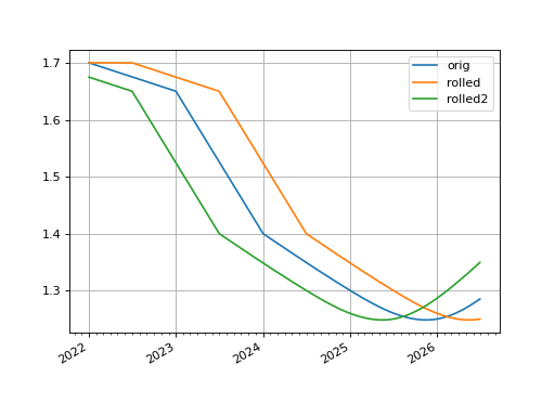
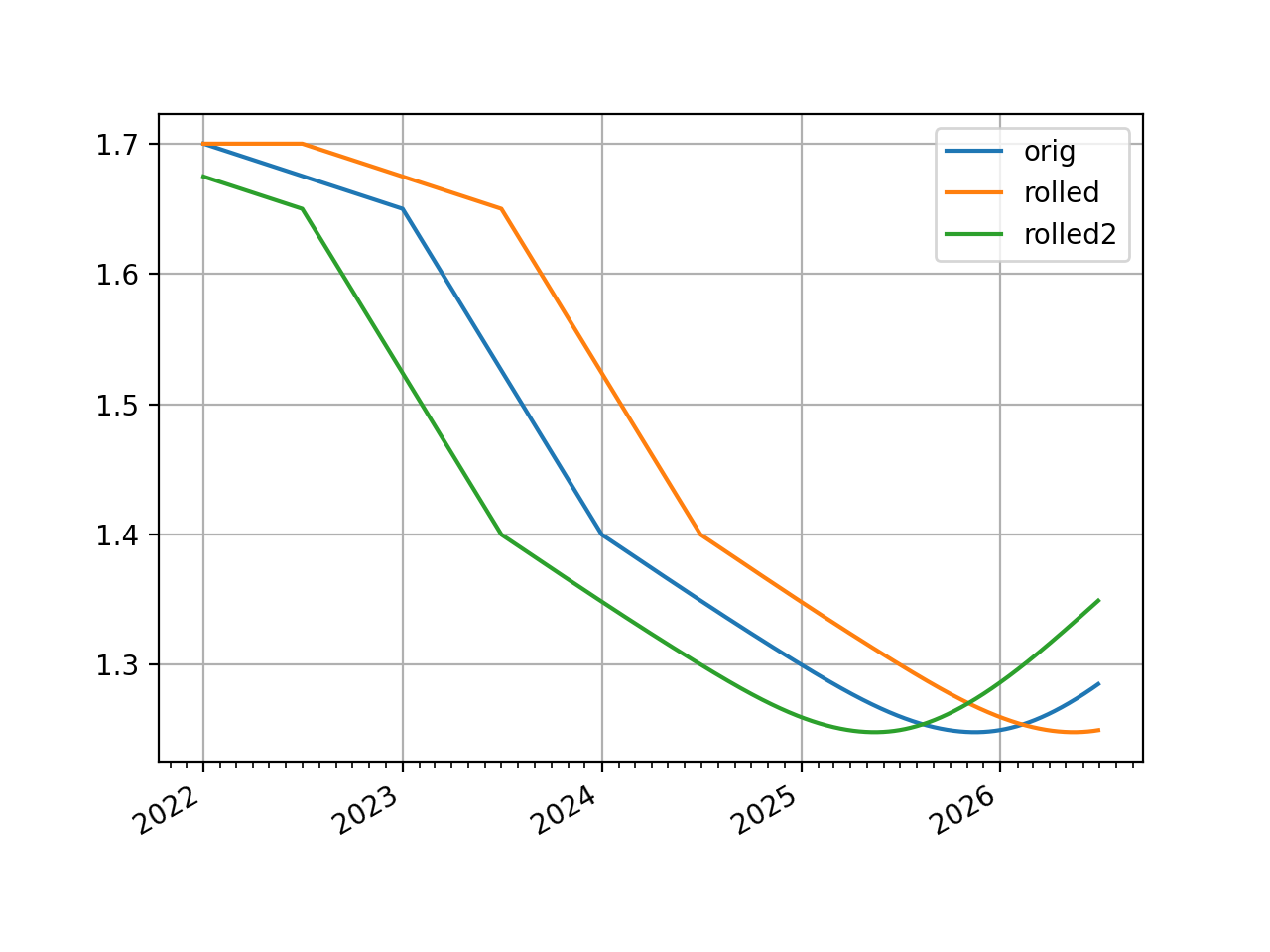
This curve adjustment is a simulation of a future state of the market where forward rates are assumed to have moved so that the present day’s curve shape is reflected in the future (or the past). This is often used in trade strategy analysis.

Parameters:

tenor (datetime or str) – The date or tenor by which to roll the curve. If a tenor, as str, will derive the datetime as measured from the initial node date. If supplying a negative tenor, or a past datetime, there is a limit to how far back the curve can be rolled - it will first roll backwards and then attempt to translate() forward to maintain the initial node date.

Return type:

Curve

Examples

The basic use of this function translates a curve forward in time and the plot demonstrates its rates are exactly the same as initially forecast.

In [1]: line_curve = LineCurve(
   ...:     nodes = {
   ...:         dt(2022, 1, 1): 1.7,
   ...:         dt(2023, 1, 1): 1.65,
   ...:         dt(2024, 1, 1): 1.4,
   ...:         dt(2025, 1, 1): 1.3,
   ...:         dt(2026, 1, 1): 1.25,
   ...:         dt(2027, 1, 1): 1.35
   ...:     },
   ...:     t = [
   ...:         dt(2024, 1, 1), dt(2024, 1, 1), dt(2024, 1, 1), dt(2024, 1, 1),
   ...:         dt(2025, 1, 1),
   ...:         dt(2026, 1, 1),
   ...:         dt(2027, 1, 1), dt(2027, 1, 1), dt(2027, 1, 1), dt(2027, 1, 1),
   ...:     ],
   ...: )
   ...: 

In [2]: rolled_curve = line_curve.roll("6m")

In [3]: rolled_curve2 = line_curve.roll("-6m")

In [4]: line_curve.plot(
   ...:     "1d",
   ...:     comparators=[rolled_curve, rolled_curve2],
   ...:     labels=["orig", "rolled", "rolled2"],
   ...:     right=dt(2026, 7, 1)
   ...: )
   ...: 
Out[4]: 
(<Figure size 640x480 with 1 Axes>,
 <Axes: >,
 [<matplotlib.lines.Line2D at 0x7f0aa513bc50>,
  <matplotlib.lines.Line2D at 0x7f0aa544af90>,
  <matplotlib.lines.Line2D at 0x7f0aa544a350>])

(Source code, png, hires.png, pdf)

shift(spread, id=None, composite=True, collateral=None)

Raise or lower the curve in parallel by a set number of basis points.

Parameters:

• spread (float, Dual, Dual2) – The number of basis points added to the existing curve.

• id (str, optional) – Set the id of the returned curve.

• composite (bool, optional) – If True will return a CompositeCurve that adds a flat curve to the existing curve. This results in slower calculations but the curve will maintain a dynamic association with the underlying curve and will change if the underlying curve changes.

• collateral (str, optional) – Designate a collateral tag for the curve which is used by other methods.

Return type:

LineCurve

Examples

In [1]: from rateslib.curves import LineCurve

In [2]: line_curve = LineCurve(
   ...:     nodes = {
   ...:         dt(2022, 1, 1): 1.7,
   ...:         dt(2023, 1, 1): 1.65,
   ...:         dt(2024, 1, 1): 1.4,
   ...:         dt(2025, 1, 1): 1.3,
   ...:         dt(2026, 1, 1): 1.25,
   ...:         dt(2027, 1, 1): 1.35
   ...:     },
   ...:     t = [
   ...:         dt(2024, 1, 1), dt(2024, 1, 1), dt(2024, 1, 1), dt(2024, 1, 1),
   ...:         dt(2025, 1, 1),
   ...:         dt(2026, 1, 1),
   ...:         dt(2027, 1, 1), dt(2027, 1, 1), dt(2027, 1, 1), dt(2027, 1, 1),
   ...:     ],
   ...: )
   ...: 

In [3]: spread_curve = line_curve.shift(25)

In [4]: line_curve.plot("1d", comparators=[spread_curve])
Out[4]: 
(<Figure size 640x480 with 1 Axes>,
 <Axes: >,
 [<matplotlib.lines.Line2D at 0x7f0aa4ce5990>,
  <matplotlib.lines.Line2D at 0x7f0aa48db250>])

(Source code, png, hires.png, pdf)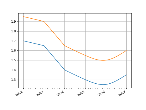

to_json()

Convert the parameters of the curve to JSON format.

Return type:

str

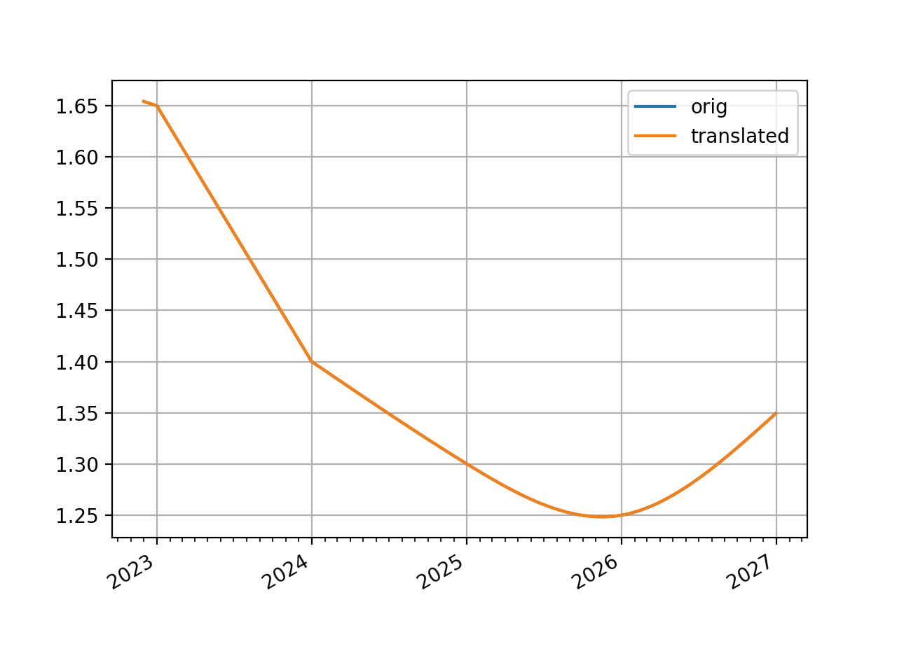
translate(start, t=False)

Create a new curve with an initial node date moved forward keeping all else constant.

This curve adjustment preserves forward curve expectations as time evolves. This method is suitable as a way to create a subsequent opening curve from a previous day’s closing curve.

Parameters:

• start (datetime) – The new initial node date for the curve, must be in the domain: (node_date[0], node_date[1]]

• t (bool) – Set to True if the initial knots of the knot sequence should be translated forward.

Return type:

Curve

Examples

The basic use of this function translates a curve forward in time and the plot demonstrates its rates are exactly the same as initially forecast.

In [1]: line_curve = LineCurve(
   ...:     nodes = {
   ...:         dt(2022, 1, 1): 1.7,
   ...:         dt(2023, 1, 1): 1.65,
   ...:         dt(2024, 1, 1): 1.4,
   ...:         dt(2025, 1, 1): 1.3,
   ...:         dt(2026, 1, 1): 1.25,
   ...:         dt(2027, 1, 1): 1.35
   ...:     },
   ...:     t = [
   ...:         dt(2024, 1, 1), dt(2024, 1, 1), dt(2024, 1, 1), dt(2024, 1, 1),
   ...:         dt(2025, 1, 1),
   ...:         dt(2026, 1, 1),
   ...:         dt(2027, 1, 1), dt(2027, 1, 1), dt(2027, 1, 1), dt(2027, 1, 1),
   ...:     ],
   ...: )
   ...: 

In [2]: translated_curve = line_curve.translate(dt(2022, 12, 1))

In [3]: line_curve.plot("1d", comparators=[translated_curve], left=dt(2022, 12, 1))
Out[3]: 
(<Figure size 640x480 with 1 Axes>,
 <Axes: >,
 [<matplotlib.lines.Line2D at 0x7f0aa5d23f50>,
  <matplotlib.lines.Line2D at 0x7f0aa5ac05d0>])

(Source code, png, hires.png, pdf)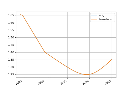

In [4]: line_curve.nodes
Out[4]: 
{datetime.datetime(2022, 1, 1, 0, 0): 1.7,
 datetime.datetime(2023, 1, 1, 0, 0): 1.65,
 datetime.datetime(2024, 1, 1, 0, 0): 1.4,
 datetime.datetime(2025, 1, 1, 0, 0): 1.3,
 datetime.datetime(2026, 1, 1, 0, 0): 1.25,
 datetime.datetime(2027, 1, 1, 0, 0): 1.35}

In [5]: translated_curve.nodes
Out[5]: 
{datetime.datetime(2022, 12, 1, 0, 0): 1.6542465753424658,
 datetime.datetime(2023, 1, 1, 0, 0): 1.65,
 datetime.datetime(2024, 1, 1, 0, 0): 1.4,
 datetime.datetime(2025, 1, 1, 0, 0): 1.3,
 datetime.datetime(2026, 1, 1, 0, 0): 1.25,
 datetime.datetime(2027, 1, 1, 0, 0): 1.35}

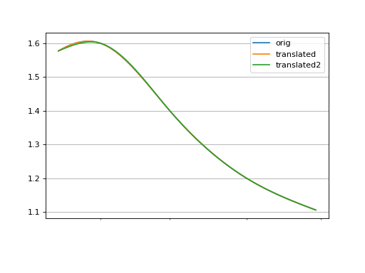
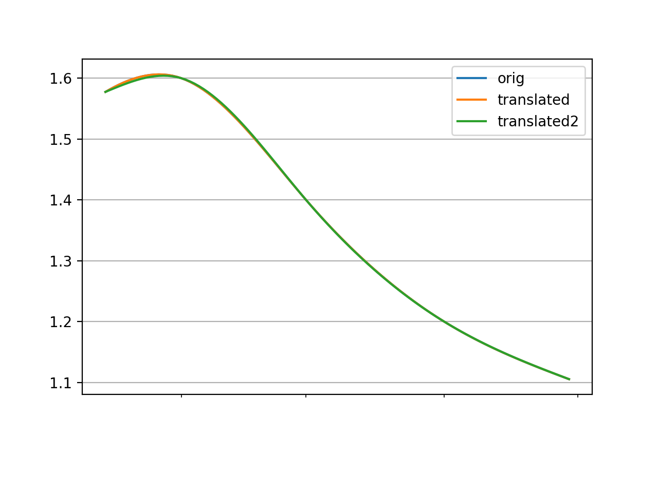
When a line curve has a cubic spline the knot dates can be preserved or translated with the t argument. Preserving the knot dates preserves the interpolation of the curve. A knot sequence for a mixed curve which begins after start will not be affected in either case.

In [6]: curve = LineCurve(
   ...:     nodes={
   ...:         dt(2022, 1, 1): 1.5,
   ...:         dt(2022, 2, 1): 1.6,
   ...:         dt(2022, 3, 1): 1.4,
   ...:         dt(2022, 4, 1): 1.2,
   ...:         dt(2022, 5, 1): 1.1,
   ...:     },
   ...:     t = [dt(2022, 1, 1), dt(2022, 1, 1), dt(2022, 1, 1), dt(2022, 1, 1),
   ...:          dt(2022, 2, 1), dt(2022, 3, 1), dt(2022, 4, 1),
   ...:          dt(2022, 5, 1), dt(2022, 5, 1), dt(2022, 5, 1), dt(2022, 5, 1)]
   ...: )
   ...: 

In [7]: translated_curve = curve.translate(dt(2022, 1, 15))

In [8]: translated_curve2 = curve.translate(dt(2022, 1, 15), t=True)

In [9]: curve.plot("1d", left=dt(2022, 1, 15), comparators=[translated_curve, translated_curve2], labels=["orig", "translated", "translated2"])
Out[9]: 
(<Figure size 640x480 with 1 Axes>,
 <Axes: >,
 [<matplotlib.lines.Line2D at 0x7f0aa5113f10>,
  <matplotlib.lines.Line2D at 0x7f0aa4b76050>,
  <matplotlib.lines.Line2D at 0x7f0aa4af70d0>])

(Source code, png, hires.png, pdf)