Curves#
The rateslib.curves module allows the fundamental Curve,
LineCurve, or IndexCurve class
to be defined with parameters (for the purpose of the user guide an IndexCurve
can be considered a Curve with minor enhancements).
These curve objects are slightly different in what they
represent and how they operate.
This module relies on the ultility modules splines and dual.
|
Curve based on DF parametrisation at given node dates with interpolation. |
|
Curve based on value parametrisation at given node dates with interpolation. |
|
A subclass of |
|
A dynamic composition of a sequence of other curves. |
|
A subclass of |
|
A dynamic composition of a sequence of other curves. |
|
Perform local interpolation between two data points. |
|
Return the interval index of a value from an ordered input list on the left side. |
Each fundamental curve type has rate(), plot(), shift(), roll() and
translate() methods. IndexCurve can also calculate
future index_value().
|
Calculate the rate on the Curve using DFs. |
|
Plot given forward tenor rates from the curve. |
|
Create a new curve by vertically adjusting the curve by a set number of basis points. |
|
Create a new curve with its shape translated in time but an identical initial node date. |
|
Create a new curve with an initial node date moved forward keeping all else constant. |
|
Return the curve value for a given date. |
|
Plot given forward tenor rates from the curve. |
|
Raise or lower the curve in parallel by a set number of basis points. |
Create a new curve with its shape translated in time |
|
|
Create a new curve with an initial node date moved forward keeping all else constant. |
Calculate the accrued value of the index from the |
The main parameter that must be supplied to either type of curve is its nodes. This
provides the curve with its degrees of freedom and represents a dict indexed by
datetimes, each with a given value. In the case of a Curve
these
values are discount factors (DFs), and in the case of
a LineCurve
these are specific values, usually rates associated with that curve.
Curve#
A Curve can only be used for interest rates.
It is a more specialised
object because of the way it is defined by discount factors (DFs). These DFs
maintain an inherent interpolation technique, which is often log-linear or log-cubic
spline. These are generally the most efficient
type of curve, and most easily parametrised, when working with compounded RFR rates.
The initial node on a Curve should always have value 1.0,
and it will not
be varied by a Solver. Curve s must
be used with
FXForwards since FX forwards calculation rely on the existence
of DFs.
LineCurves#
A LineCurve is a more general object which can be
used to represent other forms of datetime indexed values. The values maintain
interpolation
techniques where the most common are likely to be linear and splines. These are
generally quite inefficient, and more difficult to parametrise, when dealing with RFR
rates, but may be superior when dealing with legacy IBOR rates or inflation etc.
The initial node on a LineCurve can take any value and it will
be varied by a Solver.
Introduction#
To create a simple curve, with localised interpolation, minimal configuration is required.
In [1]: from rateslib import dt

In [2]: curve = Curve(
   ...:     nodes={
   ...:         dt(2022,1,1): 1.0,  # <- initial DF should always be 1.0
   ...:         dt(2023,1,1): 0.99,
   ...:         dt(2024,1,1): 0.979,
   ...:         dt(2025,1,1): 0.967,
   ...:         dt(2026,1,1): 0.956,
   ...:         dt(2027,1,1): 0.946,
   ...:     },
   ...:     interpolation="log_linear",
   ...: )
   ...:
We can also use a similar configuration for a generalised curve constructed from connecting lines between values.
In [3]: linecurve = LineCurve(
   ...:     nodes={
   ...:         dt(2022,1,1): 0.975,  # <- initial value is general
   ...:         dt(2023,1,1): 1.10,
   ...:         dt(2024,1,1): 1.22,
   ...:         dt(2025,1,1): 1.14,
   ...:         dt(2026,1,1): 1.03,
   ...:         dt(2027,1,1): 1.03,
   ...:     },
   ...:     interpolation="linear",
   ...: )
   ...:
Initial Node Date#
The initial node date for either curve type is important because it is implied
to be the date of the
construction of the curve (i.e. today’s date). Any net present
values (NPVs) may assume other features
from this initial node, e.g. the regular settlement date of securities or the value of
cashflows on derivatives. This is the reason the initial discount factor should also
be exactly 1.0 on a Curve.
Get Item#
Curves have a get item method so that DFs from a Curve
or values from a LineCurve can easily be extracted
under the curve’s specified interpolation scheme.
Note
Curve DFs (and
LineCurve values), before the curve’s initial node
date return
zero, in order to value historical cashflows at zero.
Warning
Curve DFs, and
LineCurve values, after the curve’s final node date will
return a value that is an extrapolation.
This may not be a sensible or well constrained value depending upon the
interpolation.
In [4]: curve[dt(2022, 9, 26)]
Out[4]: 0.9926477364206718

In [5]: curve[dt(1999, 12, 31)]  # <- before the curve initial node date
Out[5]: 0

In [6]: curve[dt(2032, 1, 1)]  # <- extrapolated after the curve final node date
Out[6]: 0.8975214680350941
In [7]: linecurve[dt(2022, 9, 26)]
Out[7]: 1.0667808219178083

In [8]: linecurve[dt(1999, 12, 31)]  # <- before the curve initial node date
Out[8]: 0

In [9]: linecurve[dt(2032, 1, 1)]  # <- extrapolated after the curve final node date
Out[9]: 1.03
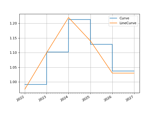
Visualization#
Visualization methods are also available via
Curve.plot() and
LineCurve.plot(). This allows the easy
inspection of curves directly. Below we demonstrate a plot highlighting the
differences between our parametrised Curve
and LineCurve.
In [10]: curve.plot(
   ....:     "1D",
   ....:     comparators=[linecurve],
   ....:     labels=["Curve", "LineCurve"]
   ....: )
   ....:
Out[10]:
(<Figure size 640x480 with 1 Axes>,
 <Axes: >,
 [<matplotlib.lines.Line2D at 0x7f0aa0c3d850>,
  <matplotlib.lines.Line2D at 0x7f0aa08d7f10>])
(Source code, png, hires.png, pdf)
Interpolation#
The available basic local interpolation options are:
“linear”: this is most suitable, and the default, for
LineCurve. Linear interpolation for DF based curves usually produces spurious underlying curves.“log_linear”: this is most suitable, and the default, for
Curve. It produces overnight rates that are constant betweennodes. This is not usually suitable forLineCurve.“linear_zero_rate”: this is a legacy option for linearly interpolating continuously compounded zero rates, and is only suitable for
Curve, but it is not recommended and tends also to produce spurious underlying curves.“flat_forward”: this is only suitable for
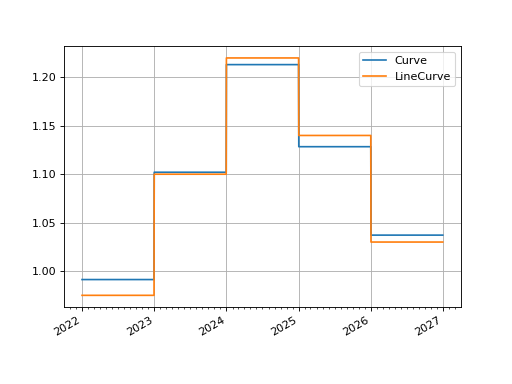
LineCurve, and it maintains the previous value betweennodes. It will produce a stepped curve similar to aCurvewith “log_linear” interpolation.“flat_backward”: same as above but in reverse.
In [11]: linecurve.interpolation = "flat_forward"

In [12]: curve.plot("1D", comparators=[linecurve], labels=["Curve", "LineCurve"])
Out[12]:
(<Figure size 640x480 with 1 Axes>,
 <Axes: >,
 [<matplotlib.lines.Line2D at 0x7f0aa178bc90>,
  <matplotlib.lines.Line2D at 0x7f0aa117c510>])
(Source code, png, hires.png, pdf)
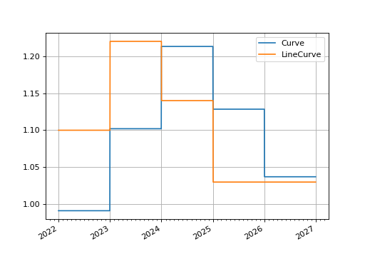
interpolation can also be specified as a user defined function. It must
have the argument signature (date, nodes) where nodes are passed internally as
those copied from the curve.
In [13]: from rateslib.curves import index_left

In [14]: def flat_backward(x, nodes):
   ....:     """Project the rightmost node value as opposed to leftmost."""
   ....:     node_dates = [key for key in nodes.keys()]
   ....:     if x < node_dates[0]:
   ....:         return 0  # then date is in the past and DF is zero
   ....:     l_index = index_left(node_dates, len(node_dates), x)
   ....:     return nodes[node_dates[l_index + 1]]
   ....:

In [15]: linecurve.interpolation = flat_backward

In [16]: curve.plot("1D", comparators=[linecurve], labels=["Curve", "LineCurve"])
Out[16]:
(<Figure size 640x480 with 1 Axes>,
 <Axes: >,
 [<matplotlib.lines.Line2D at 0x7f0aa01226d0>,
  <matplotlib.lines.Line2D at 0x7f0aa00f3f50>])
(Source code, png, hires.png, pdf)
Spline Interpolation#
There is also an option to interpolate with a cubic polynomial spline.
If applying spline interpolation to a Curve then it is
applied logarithmically resulting in a log-cubic spline over DFs.
If it is applied to a LineCurve then it results in a
standard cubic spline over values.
In order to instruct this mode of interpolation a knot sequence is required
as the t argument. This is a list of datetimes and follows the
appropriate mathematical convention for such sequences
(see pp splines).
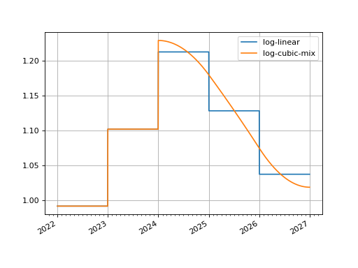
Mixed Interpolation#
Prior to the initial knot in the sequence the local interpolation method is used. This allows curves to be constructed with a mixed interpolation in two parts of the curve. This is common practice for interest rate curves usually with a log-linear short end and a log-cubic spline longer end.
In [17]: mixed_curve = Curve(
   ....:     nodes={
   ....:         dt(2022,1,1): 1.0,
   ....:         dt(2023,1,1): 0.99,
   ....:         dt(2024,1,1): 0.979,
   ....:         dt(2025,1,1): 0.967,
   ....:         dt(2026,1,1): 0.956,
   ....:         dt(2027,1,1): 0.946,
   ....:     },
   ....:     interpolation="log_linear",
   ....:     t = [dt(2024,1,1), dt(2024,1,1), dt(2024,1,1), dt(2024,1,1),
   ....:          dt(2025,1,1),
   ....:          dt(2026,1,1),
   ....:          dt(2027,1,1), dt(2027,1,1), dt(2027,1,1), dt(2027,1,1)]
   ....: )
   ....:

In [18]: curve.plot("1D", comparators=[mixed_curve], labels=["log-linear", "log-cubic-mix"])
Out[18]:
(<Figure size 640x480 with 1 Axes>,
 <Axes: >,
 [<matplotlib.lines.Line2D at 0x7f0a9ffbcfd0>,
  <matplotlib.lines.Line2D at 0x7f0a9ff6ded0>])
(Source code, png, hires.png, pdf)
IBOR or RFR#
The different Instruments in rateslib may require
different interest rate index types, be it IBOR or RFR based. These are
fundamentally different and require care dependent on
which curve type: Curve or
LineCurve is used. This is also similar to fixing input
for FloatPeriod (see here).
Curve Type |
RFR Based |
IBOR Based |
|---|---|---|
DFs are value date based. For an RFR rate applicable between a start and end date, the start and end date DFs will reflect this rate, regardless of the publication timeframe of the rate. |
DFs are value date based. For an IBOR rate applicable between a start and end date, the start and end date DFs will reflect this rate, regardless of the publication timeframe of the rate. |
|
Rates are labelled by reference value date, not publication date. |
Rates are labelled by publication date, not reference value date. |
Since DF based curves behave similarly for each index type we will give an example
of constructing an IRS under the different methods.
For an RFR curve the nodes values are by reference date. The 3.0% value which
is applicable between the reference date of 2nd Jan ‘22 and end date 3rd Jan ‘22,
is indexed according to the 2nd Jan ‘22.
In [19]: rfr_curve = LineCurve(
   ....:     nodes={
   ....:         dt(2022, 1, 1): 2.0,
   ....:         dt(2022, 1, 2): 3.0,
   ....:         dt(2022, 1, 3): 4.0
   ....:     }
   ....: )
   ....:

In [20]: irs = IRS(
   ....:     dt(2022, 1, 2),
   ....:     "1d",
   ....:     "A",
   ....:     leg2_fixing_method="rfr_payment_delay"
   ....: )
   ....:

In [21]: irs.rate(rfr_curve)
Out[21]: 3.0000000000036664
For an IBOR curve the nodes values are by publication date. The curve below has a
lag of 2 business days. and the publication on 1st Jan ‘22 is applicable to the
reference value date of 3rd Jan.
In [22]: ibor_curve = LineCurve(
   ....:     nodes={
   ....:         dt(2022, 1, 1): 2.5,
   ....:         dt(2022, 1, 2): 3.5,
   ....:         dt(2022, 1, 3): 4.5
   ....:     }
   ....: )
   ....:

In [23]: irs = IRS(
   ....:     dt(2022, 1, 3),
   ....:     "3m",
   ....:     "A",
   ....:     leg2_fixing_method="ibor",
   ....:     leg2_method_param=2
   ....: )
   ....:

In [24]: irs.rate(ibor_curve)
Out[24]: 2.5