ProxyCurve#
- class rateslib.curves.ProxyCurve(cashflow, collateral, fx_forwards, convention=None, modifier=False, calendar=False, id=None)#
Bases:
CurveA subclass of
Curvewhich returns dynamic DFs based on other curves related viaFXForwardsparity.- Parameters:
cashflow (str) – The currency in which cashflows are represented (3-digit code).
collateral (str) – The currency of the CSA against which cashflows are collateralised (3-digit code).
fx_forwards (FXForwards) – The
FXForwardsobject which contains the relating FX information and the availableCurves.convention (str) – The day count convention used for calculating rates. If None defaults to the convention in the local cashflow currency.
modifier (str, optional) – The modification rule, in {“F”, “MF”, “P”, “MP”}, for determining rates. If False will default to the modifier in the local cashflow currency.
calendar (calendar or str, optional) – The holiday calendar object to use. If str, lookups named calendar from static data. Used for determining rates. If False will default to the calendar in the local cashflow currency.
id (str, optional, set by Default) – The unique identifier to distinguish between curves in a multi-curve framework.
Notes
The DFs returned are calculated via the chaining method and the below formula, relating the DF curve in the local collateral currency and FX forward rates.
\[w_{dom:for,i} = \frac{f_{DOMFOR,i}}{F_{DOMFOR,0}} v_{for:for,i}\]The returned curve contains contrived methods to calculate this dynamically and efficiently from the combination of curves and FX rates that are available within the given
FXForwardsinstance.Attributes Summary
Methods Summary
copy()Create an identical copy of the curve object.
csolve()Solves and sets the coefficients,
c, of thePPSpline.Not implemented for
ProxyCurves.plot(tenor[, right, left, comparators, ...])Plot given forward tenor rates from the curve.
rate(effective, termination[, modifier, ...])Calculate the rate on the Curve using DFs.
roll(tenor)Create a new curve with its shape translated in time but an identical initial node date.
shift(spread[, id, composite, collateral])Create a new curve by vertically adjusting the curve by a set number of basis points.
to_json()Not implemented for
ProxyCurves.translate(start[, t])Create a new curve with an initial node date moved forward keeping all else constant.
Attributes Documentation
- collateral = None#
Methods Documentation
- csolve()#
Solves and sets the coefficients,
c, of thePPSpline.- Return type:
None
Notes
Only impacts curves which have a knot sequence,
t, and aPPSpline. Only solves ifcnot given at curve initialisation.Uses the
spline_endpointsattribute on the class to determine the solving method.
- from_json()#
Not implemented for
ProxyCurves.
- plot(tenor, right=NoInput.blank, left=NoInput.blank, comparators=[], difference=False, labels=[])#
Plot given forward tenor rates from the curve.
- Parameters:
tenor (str) – The tenor of the forward rates to plot, e.g. “1D”, “3M”.
right (datetime or str, optional) – The right bound of the graph. If given as str should be a tenor format defining a point measured from the initial node date of the curve. Defaults to the final node of the curve minus the
tenor.left (datetime or str, optional) – The left bound of the graph. If given as str should be a tenor format defining a point measured from the initial node date of the curve. Defaults to the initial node of the curve.
comparators (list[Curve]) – A list of curves which to include on the same plot as comparators.
difference (bool) – Whether to plot as comparator minus base curve or outright curve levels in plot. Default is False.
labels (list[str]) – A list of strings associated with the plot and comparators. Must be same length as number of plots.
- Returns:
(fig, ax, line)
- Return type:
Matplotlib.Figure, Matplotplib.Axes, Matplotlib.Lines2D
- rate(effective, termination, modifier=NoInput.blank, float_spread=None, spread_compound_method=None)#
Calculate the rate on the Curve using DFs.
If rates are sought for dates prior to the initial node of the curve None will be returned.
- Parameters:
effective (datetime) – The start date of the period for which to calculate the rate.
termination (datetime or str) – The end date of the period for which to calculate the rate.
modifier (str, optional) – The day rule if determining the termination from tenor. If False is determined from the Curve modifier.
float_spread (float, optional) – A float spread can be added to the rate in certain cases.
spread_compound_method (str in {"none_simple", "isda_compounding"}) – The method if adding a float spread. If “none_simple” is used this results in an exact calculation. If “isda_compounding” or “isda_flat_compounding” is used this results in an approximation.
- Return type:
Notes
Calculating rates from a curve implies that the conventions attached to the specific index, e.g. USD SOFR, or GBP SONIA, are applicable and these should be set at initialisation of the
Curve. Thus, the convention used to calculate therateis taken from theCurvefrom whichrateis called.modifieris only used if a tenor is given as the termination.Major indexes, such as legacy IBORs, and modern RFRs typically use a
conventionwhich is either “Act365F” or “Act360”. These conventions do not need additional parameters, such as the termination of a leg, the frequency or a leg or whether it is a stub to calculate a DCF.Adding Floating Spreads
An optimised method for adding floating spreads to a curve rate is provided. This is quite restrictive and mainly used internally to facilitate other parts of the library.
When
spread_compound_methodis “none_simple” the spread is a simple linear addition.When using “isda_compounding” or “isda_flat_compounding” the curve is assumed to be comprised of RFR rates and an approximation is used to derive to total rate.
Examples
In [10]: curve_act365f = Curve(
   ....:     nodes={
   ....:         dt(2022, 1, 1): 1.0,
   ....:         dt(2022, 2, 1): 0.98,
   ....:         dt(2022, 3, 1): 0.978,
   ....:     },
   ....:     convention='Act365F'
   ....: )
   ....:

In [11]: curve_act365f.rate(dt(2022, 2, 1), dt(2022, 3, 1))
Out[11]: 2.6657902424774402
Using a different convention will result in a different rate:
In [12]: curve_act360 = Curve(
   ....:     nodes={
   ....:         dt(2022, 1, 1): 1.0,
   ....:         dt(2022, 2, 1): 0.98,
   ....:         dt(2022, 3, 1): 0.978,
   ....:     },
   ....:     convention='Act360'
   ....: )
   ....:

In [13]: curve_act360.rate(dt(2022, 2, 1), dt(2022, 3, 1))
Out[13]: 2.6292725679229547
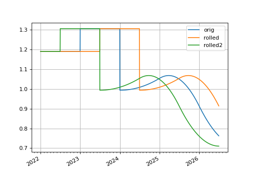
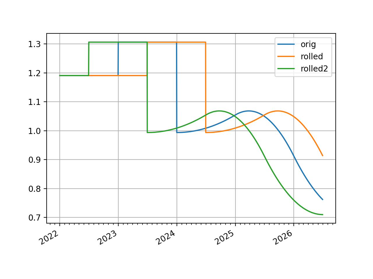
- roll(tenor)#
Create a new curve with its shape translated in time but an identical initial node date.
This curve adjustment is a simulation of a future state of the market where forward rates are assumed to have moved so that the present day’s curve shape is reflected in the future (or the past). This is often used in trade strategy analysis.
- Parameters:
tenor (datetime or str) – The date or tenor by which to roll the curve. If a tenor, as str, will derive the datetime as measured from the initial node date. If supplying a negative tenor, or a past datetime, there is a limit to how far back the curve can be rolled - it will first roll backwards and then attempt to
translate()forward to maintain the initial node date.- Return type:
Examples
The basic use of this function translates a curve forward in time and the plot demonstrates its rates are exactly the same as initially forecast.
In [14]: curve = Curve(
   ....:     nodes = {
   ....:         dt(2022, 1, 1): 1.0,
   ....:         dt(2023, 1, 1): 0.988,
   ....:         dt(2024, 1, 1): 0.975,
   ....:         dt(2025, 1, 1): 0.965,
   ....:         dt(2026, 1, 1): 0.955,
   ....:         dt(2027, 1, 1): 0.9475
   ....:     },
   ....:     t = [
   ....:         dt(2024, 1, 1), dt(2024, 1, 1), dt(2024, 1, 1), dt(2024, 1, 1),
   ....:         dt(2025, 1, 1),
   ....:         dt(2026, 1, 1),
   ....:         dt(2027, 1, 1), dt(2027, 1, 1), dt(2027, 1, 1), dt(2027, 1, 1),
   ....:     ],
   ....: )
   ....:

In [15]: rolled_curve = curve.roll("6m")

In [16]: rolled_curve2 = curve.roll("-6m")

In [17]: curve.plot(
   ....:     "1d",
   ....:     comparators=[rolled_curve, rolled_curve2],
   ....:     labels=["orig", "rolled", "rolled2"],
   ....:     right=dt(2026, 7, 1),
   ....: )
   ....:
Out[17]:
(<Figure size 640x480 with 1 Axes>,
 <Axes: >,
 [<matplotlib.lines.Line2D at 0x7f0aa462f6d0>,
  <matplotlib.lines.Line2D at 0x7f0aa468fad0>,
  <matplotlib.lines.Line2D at 0x7f0aa46a04d0>])
(
Source code,png,hires.png,pdf)
- shift(spread, id=None, composite=True, collateral=None)#
Create a new curve by vertically adjusting the curve by a set number of basis points.
This curve adjustment preserves the shape of the curve but moves it up or down as a translation. This method is suitable as a way to assess value changes of instruments when a parallel move higher or lower in yields is predicted.
- Parameters:
spread (float, Dual, Dual2) – The number of basis points added to the existing curve.
id (str, optional) – Set the id of the returned curve.
composite (bool, optional) – If True will return a CompositeCurve that adds a flat curve to the existing curve. This results in slower calculations but the curve will maintain a dynamic association with the underlying curve and will change if the underlying curve changes.
collateral (str, optional) – Designate a collateral tag for the curve which is used by other methods.
- Return type:
Examples
In [18]: from rateslib.curves import Curve
In [19]: curve = Curve(
   ....:     nodes = {
   ....:         dt(2022, 1, 1): 1.0,
   ....:         dt(2023, 1, 1): 0.988,
   ....:         dt(2024, 1, 1): 0.975,
   ....:         dt(2025, 1, 1): 0.965,
   ....:         dt(2026, 1, 1): 0.955,
   ....:         dt(2027, 1, 1): 0.9475
   ....:     },
   ....:     t = [
   ....:         dt(2024, 1, 1), dt(2024, 1, 1), dt(2024, 1, 1), dt(2024, 1, 1),
   ....:         dt(2025, 1, 1),
   ....:         dt(2026, 1, 1),
   ....:         dt(2027, 1, 1), dt(2027, 1, 1), dt(2027, 1, 1), dt(2027, 1, 1),
   ....:     ],
   ....: )
   ....:

In [20]: shifted_curve = curve.shift(25)

In [21]: curve.plot("1d", comparators=[shifted_curve], labels=["orig", "shift"])
Out[21]:
(<Figure size 640x480 with 1 Axes>,
 <Axes: >,
 [<matplotlib.lines.Line2D at 0x7f0aa443a6d0>,
  <matplotlib.lines.Line2D at 0x7f0aa4332dd0>])
(
Source code,png,hires.png,pdf)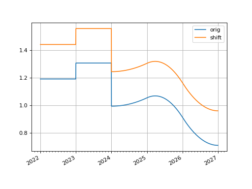
- to_json()#
Not implemented for
ProxyCurves. :return:
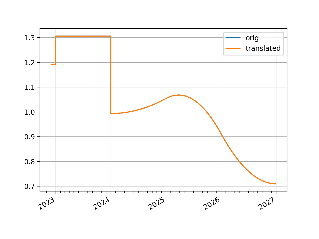
- translate(start, t=False)#
Create a new curve with an initial node date moved forward keeping all else constant.
This curve adjustment preserves forward curve expectations as time evolves. This method is suitable as a way to create a subsequent opening curve from a previous day’s closing curve.
- Parameters:
start (datetime) – The new initial node date for the curve, must be in the domain: (node_date[0], node_date[1]]
t (bool) – Set to True if the initial knots of the knot sequence should be translated forward.
- Return type:
Examples
The basic use of this function translates a curve forward in time and the plot demonstrates its rates are exactly the same as initially forecast.
In [22]: curve = Curve(
   ....:     nodes = {
   ....:         dt(2022, 1, 1): 1.0,
   ....:         dt(2023, 1, 1): 0.988,
   ....:         dt(2024, 1, 1): 0.975,
   ....:         dt(2025, 1, 1): 0.965,
   ....:         dt(2026, 1, 1): 0.955,
   ....:         dt(2027, 1, 1): 0.9475
   ....:     },
   ....:     t = [
   ....:         dt(2024, 1, 1), dt(2024, 1, 1), dt(2024, 1, 1), dt(2024, 1, 1),
   ....:         dt(2025, 1, 1),
   ....:         dt(2026, 1, 1),
   ....:         dt(2027, 1, 1), dt(2027, 1, 1), dt(2027, 1, 1), dt(2027, 1, 1),
   ....:     ],
   ....: )
   ....:

In [23]: translated_curve = curve.translate(dt(2022, 12, 1))

In [24]: curve.plot(
   ....:     "1d",
   ....:     comparators=[translated_curve],
   ....:     labels=["orig", "translated"],
   ....:     left=dt(2022, 12, 1),
   ....: )
   ....:
Out[24]:
(<Figure size 640x480 with 1 Axes>,
 <Axes: >,
 [<matplotlib.lines.Line2D at 0x7f0aa5110490>,
  <matplotlib.lines.Line2D at 0x7f0aa4bac1d0>])
(
Source code,png,hires.png,pdf)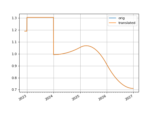
In [25]: curve.nodes
Out[25]:
{datetime.datetime(2022, 1, 1, 0, 0): 1.0,
 datetime.datetime(2023, 1, 1, 0, 0): 0.988,
 datetime.datetime(2024, 1, 1, 0, 0): 0.975,
 datetime.datetime(2025, 1, 1, 0, 0): 0.965,
 datetime.datetime(2026, 1, 1, 0, 0): 0.955,
 datetime.datetime(2027, 1, 1, 0, 0): 0.9475}

In [26]: translated_curve.nodes
Out[26]:
{datetime.datetime(2022, 12, 1, 0, 0): 1.0,
 datetime.datetime(2023, 1, 1, 0, 0): 0.9989751829682344,
 datetime.datetime(2024, 1, 1, 0, 0): 0.9858307726660208,
 datetime.datetime(2025, 1, 1, 0, 0): 0.9757196878181642,
 datetime.datetime(2026, 1, 1, 0, 0): 0.9656086029703076,
 datetime.datetime(2027, 1, 1, 0, 0): 0.9580252893344151}
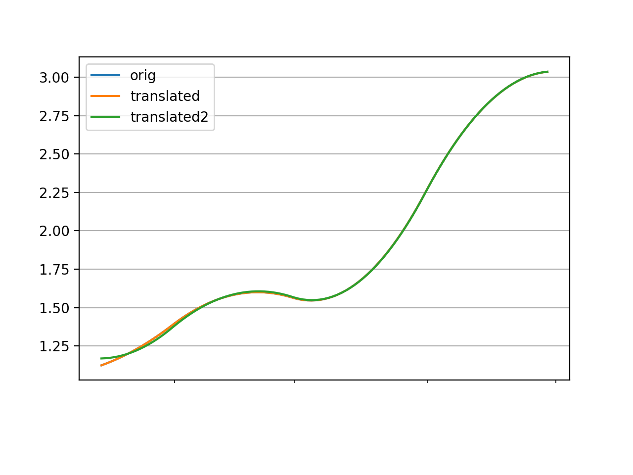
When a curve has a log-cubic spline the knot dates can be preserved or translated with the
targument. Preserving the knot dates preserves the interpolation of the curve. A knot sequence for a mixed curve which begins afterstartwill not be affected in either case.In [27]: curve = Curve( ....: nodes={ ....: dt(2022, 1, 1): 1.0, ....: dt(2022, 2, 1): 0.999, ....: dt(2022, 3, 1): 0.9978, ....: dt(2022, 4, 1): 0.9963, ....: dt(2022, 5, 1): 0.9940 ....: }, ....: t = [dt(2022, 1, 1), dt(2022, 1, 1), dt(2022, 1, 1), dt(2022, 1, 1), ....: dt(2022, 2, 1), dt(2022, 3, 1), dt(2022, 4, 1), ....: dt(2022, 5, 1), dt(2022, 5, 1), dt(2022, 5, 1), dt(2022, 5, 1)] ....: ) ....: In [28]: translated_curve = curve.translate(dt(2022, 1, 15)) In [29]: translated_curve2 = curve.translate(dt(2022, 1, 15), t=True) In [30]: curve.plot("1d", left=dt(2022, 1, 15), comparators=[translated_curve, translated_curve2], labels=["orig", "translated", "translated2"]) Out[30]: (<Figure size 640x480 with 1 Axes>, <Axes: >, [<matplotlib.lines.Line2D at 0x7f0aa4f66750>, <matplotlib.lines.Line2D at 0x7f0aa505f410>, <matplotlib.lines.Line2D at 0x7f0aa505dfd0>])
(
Source code,png,hires.png,pdf)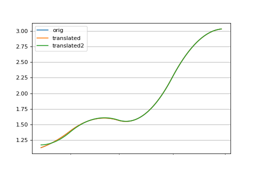