Constructing Curves

Rateslib has six different curve classes. Three of these are fundamental base curves of different types and for different purposes. Three are objects which are constructed via references to other curves to allow certain combinations.

The three fundamental curve classes are:

rateslib.curves.Curve(nodes, *[, ...])	Curve based on DF parametrisation at given node dates with interpolation.
rateslib.curves.LineCurve(*args, **kwargs)	Curve based on value parametrisation at given node dates with interpolation.
rateslib.curves.IndexCurve(*args[, ...])	A subclass of Curve with an index_base value for index calculations.

The remaining, more complex, combination classes are:

rateslib.curves.CompositeCurve(curves[, id])	A dynamic composition of a sequence of other curves.
rateslib.curves.ProxyCurve(cashflow, ...[, ...])	A subclass of Curve which returns dynamic DFs based on other curves related via FXForwards parity.
rateslib.curves.MultiCsaCurve(curves[, id, ...])	A dynamic composition of a sequence of other curves.

In rateslib defining curves and then solving them with calibrating instruments are two separate processes. This provides maximal flexibility whilst providing a process that is fully generalised and consistent throughout.

Warning

Rateslib does not bootstrap. Bootstrapping is an analytical process that determines curve parameters sequentially and exactly by solving a series of equations for a well defined set of parameters and instruments. All curves that can be bootstrapped can also be solved by a numerical optimisation routine.

The following pages describe these two processes.

• Curves
• Solver

The below provides a basic introduction, exemplifying how a SOFR curve, which might otherwise be bootstrapped, can be constructed in rateslib using the generalised process of:

• defining the Curves,

• defining the calibrating Instruments,

• combining in the Solver with target market prices.

In [1]: from rateslib.curves import Curve

In [2]: from rateslib.solver import Solver

In [3]: from rateslib.instruments import IRS

In [4]: from rateslib import dt

In [5]: sofr = Curve(
   ...:     nodes={
   ...:         dt(2022, 1, 1): 1.0,
   ...:         dt(2022, 2, 1): 1.0,  # 1M node
   ...:         dt(2022, 3, 1): 1.0,  # 2M node
   ...:         dt(2022, 4, 1): 1.0,  # 3M node
   ...:         dt(2022, 7, 1): 1.0,  # 6M node
   ...:         dt(2023, 1, 1): 1.0,  # 1Y node
   ...:         dt(2024, 1, 1): 1.0,  # 2Y node
   ...:     },
   ...:     id="sofr",
   ...: )
   ...: 

In [6]: instruments = [
   ...:     IRS(dt(2022, 1, 1), "1M", "A", curves="sofr"),
   ...:     IRS(dt(2022, 1, 1), "2M", "A", curves="sofr"),
   ...:     IRS(dt(2022, 1, 1), "3M", "A", curves="sofr"),
   ...:     IRS(dt(2022, 1, 1), "6M", "A", curves="sofr"),
   ...:     IRS(dt(2022, 1, 1), "1Y", "A", curves="sofr"),
   ...:     IRS(dt(2022, 1, 1), "2Y", "A", curves="sofr"),
   ...: ]
   ...: 

In [7]: rates = [2.4, 2.55, 2.7, 3.1, 3.6, 3.9]

In [8]: solver = Solver(
   ...:     curves=[sofr],
   ...:     instruments=instruments,
   ...:     s=rates,
   ...: )
   ...: 
SUCCESS: `func_tol` reached after 4 iterations (levenberg_marquardt), `f_val`: 5.016431301425405e-16, `time`: 0.0112s

In [9]: sofr.nodes
Out[9]: 
{datetime.datetime(2022, 1, 1, 0, 0): <Dual: 1.000000, (sofr0, sofr1, sofr2, ...), [1.0, 0.0, 0.0, ...]>,
 datetime.datetime(2022, 2, 1, 0, 0): <Dual: 0.997938, (sofr0, sofr1, sofr2, ...), [0.0, 1.0, 0.0, ...]>,
 datetime.datetime(2022, 3, 1, 0, 0): <Dual: 0.995838, (sofr0, sofr1, sofr2, ...), [0.0, 0.0, 1.0, ...]>,
 datetime.datetime(2022, 4, 1, 0, 0): <Dual: 0.993295, (sofr0, sofr1, sofr2, ...), [0.0, 0.0, 0.0, ...]>,
 datetime.datetime(2022, 7, 1, 0, 0): <Dual: 0.984653, (sofr0, sofr1, sofr2, ...), [0.0, 0.0, 0.0, ...]>,
 datetime.datetime(2023, 1, 1, 0, 0): <Dual: 0.964785, (sofr0, sofr1, sofr2, ...), [0.0, 0.0, 0.0, ...]>,
 datetime.datetime(2024, 1, 1, 0, 0): <Dual: 0.925264, (sofr0, sofr1, sofr2, ...), [0.0, 0.0, 0.0, ...]>}

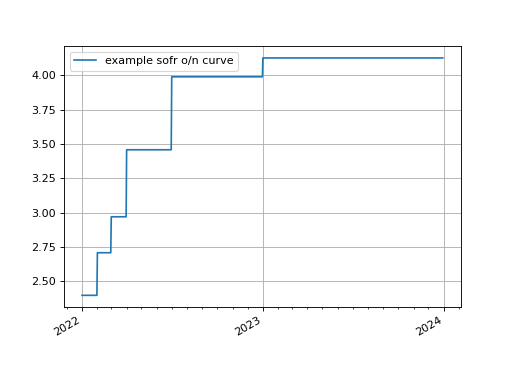
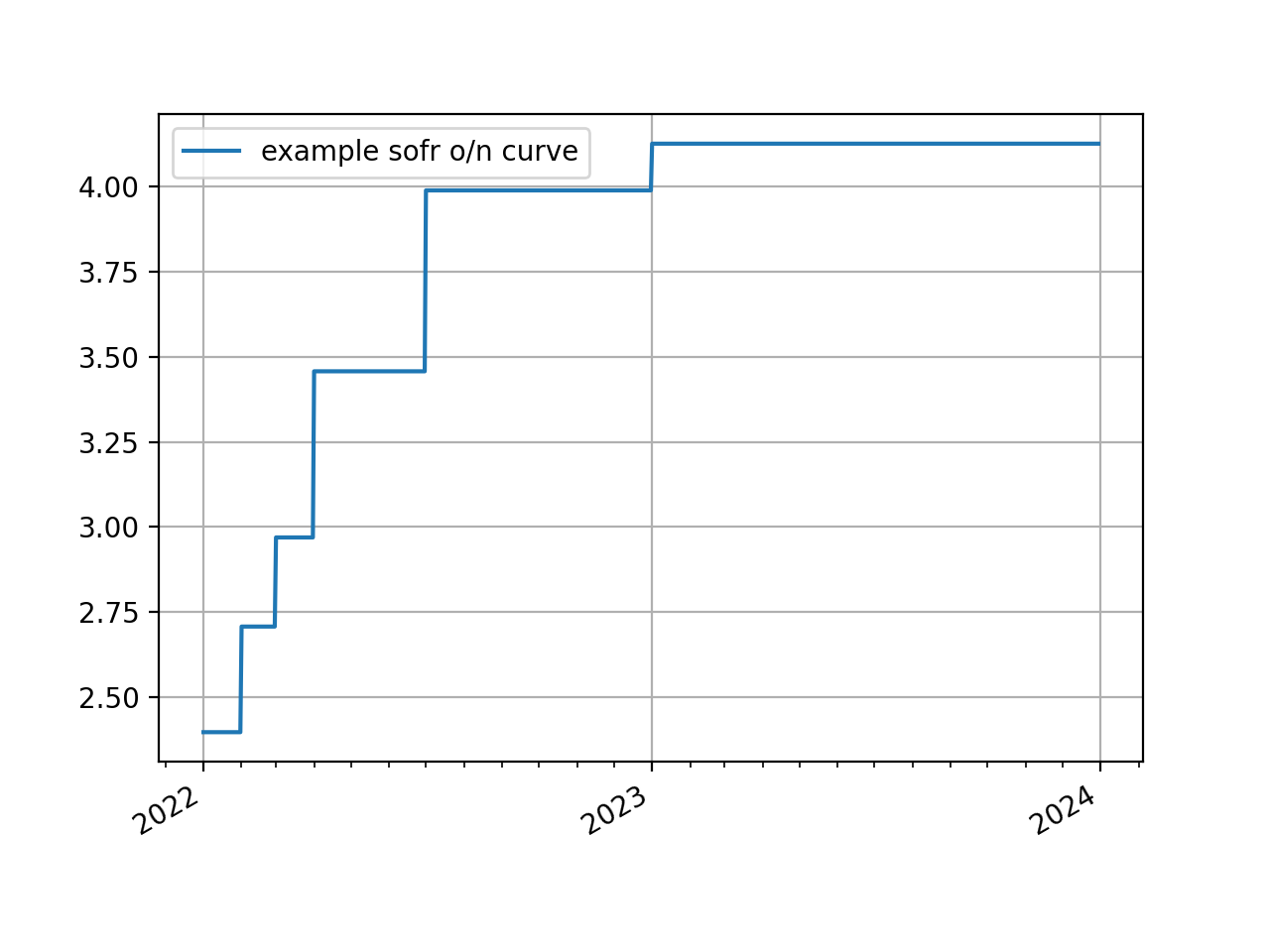
In [10]: sofr.plot("1d", labels=["example sofr o/n curve"])
Out[10]: 
(<Figure size 640x480 with 1 Axes>,
 <Axes: >,
 [<matplotlib.lines.Line2D at 0x7f90d104be50>])

(Source code, png, hires.png, pdf)