Curve#
- class rateslib.curves.Curve(nodes, *, interpolation=NoInput.blank, t=NoInput.blank, c=NoInput.blank, endpoints=NoInput.blank, id=NoInput.blank, convention=NoInput.blank, modifier=NoInput.blank, calendar=NoInput.blank, ad=0, **kwargs)#
Bases:
_SerializeCurve based on DF parametrisation at given node dates with interpolation.
- Parameters:
nodes (dict[datetime: float]) – Parameters of the curve denoted by a node date and a corresponding DF at that point.
interpolation (str or callable) – The interpolation used in the non-spline section of the curve. That is the part of the curve between the first node in
nodesand the first knot int. If a callable, this allows a user-defined interpolation scheme, and this must have the signaturemethod(date, nodes), wheredateis the datetime whose DF will be returned andnodesis as above and is passed to the callable.t (list[datetime], optional) – The knot locations for the B-spline log-cubic interpolation section of the curve. If None all interpolation will be done by the local method specified in
interpolation.c (list[float], optional) – The B-spline coefficients used to define the log-cubic spline. If not given, which is the expected case, uses
csolve()to calculate these automatically.endpoints (str or list, optional) – The left and right endpoint constraint for the spline solution. Valid values are in {“natural”, “not_a_knot”}. If a list, supply the left endpoint then the right endpoint.
id (str, optional, set by Default) – The unique identifier to distinguish between curves in a multicurve framework.
convention (str, optional, set by Default) – The convention of the curve for determining rates. Please see
dcf()for all available options.modifier (str, optional) – The modification rule, in {“F”, “MF”, “P”, “MP”}, for determining rates.
calendar (calendar or str, optional) – The holiday calendar object to use. If str, looks up named calendar from static data. Used for determining rates.
ad (int in {0, 1, 2}, optional) – Sets the automatic differentiation order. Defines whether to convert node values to float,
DualorDual2. It is advised against using this setting directly. It is mainly used internally.
Notes
This curve type is discount factor (DF) based and is parametrised by a set of (date, DF) pairs set as
nodes. The initial node date of the curve is defined to be today and should always have a DF of precisely 1.0. The initial DF will not be affected by aSolver.Intermediate DFs are determined through
interpolation. If local interpolation is adopted a DF for an arbitrary date is dependent only on its immediately neighbouring nodes via the interpolation routine. Available options are:“log_linear” (default for this curve type)
“linear_index”
And also the following which are not recommended for this curve type:
“linear”,
“linear_zero_rate”,
“flat_forward”,
“flat_backward”,
Global interpolation in the form of a log-cubic spline is also configurable with the parameters
t,candendpoints. See splines for instruction of knot sequence calibration. Values before the first knot intwill be determined through the local interpolation method.For defining rates by a given tenor, the
modifierandcalendararguments will be used. For correct scaling of the rate aconventionis attached to the curve, which is usually one of “Act360” or “Act365F”.Examples
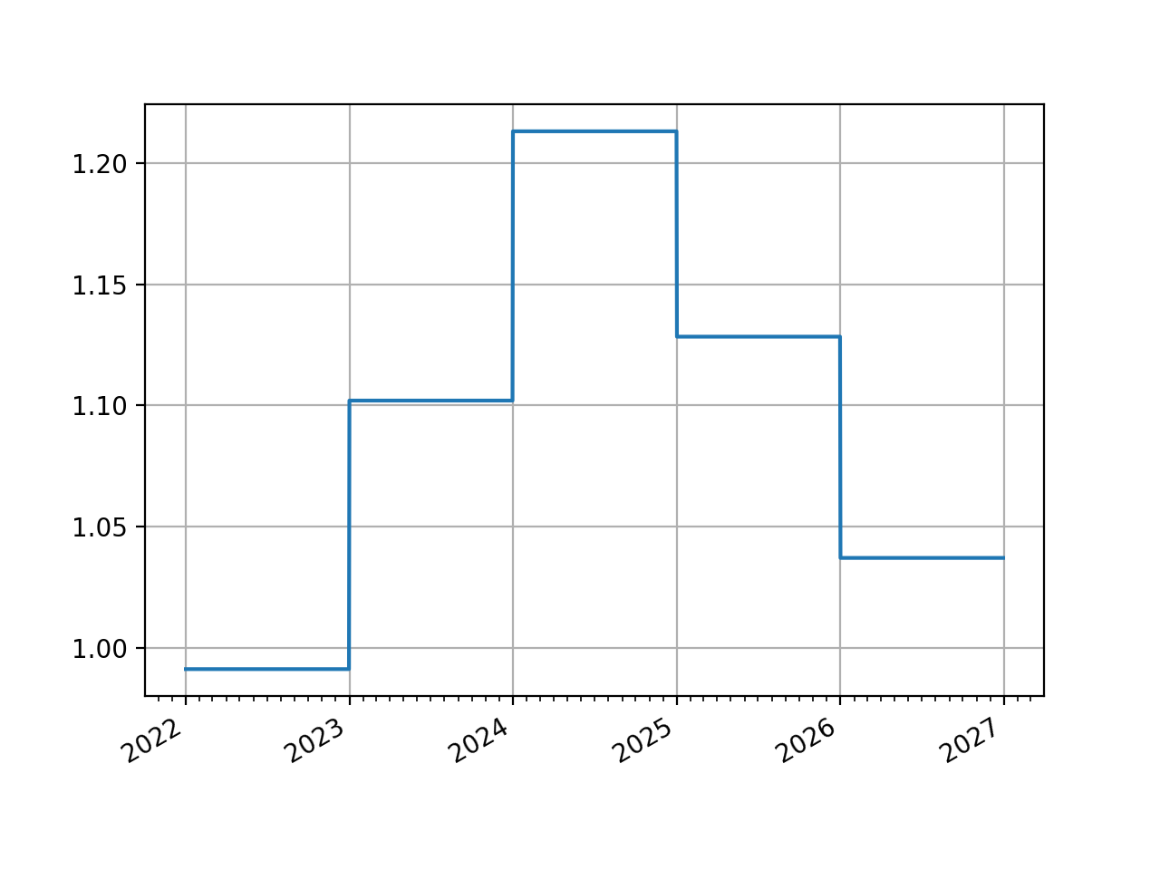
In [1]: curve = Curve(
   ...:     nodes={
   ...:         dt(2022,1,1): 1.0,  # <- initial DF should always be 1.0
   ...:         dt(2023,1,1): 0.99,
   ...:         dt(2024,1,1): 0.979,
   ...:         dt(2025,1,1): 0.967,
   ...:         dt(2026,1,1): 0.956,
   ...:         dt(2027,1,1): 0.946,
   ...:     },
   ...:     interpolation="log_linear",
   ...: )
   ...:

In [2]: curve.plot("1d")
Out[2]:
(<Figure size 640x480 with 1 Axes>,
 <Axes: >,
 [<matplotlib.lines.Line2D at 0x7f0aa52abb50>])
(
Source code,png,hires.png,pdf)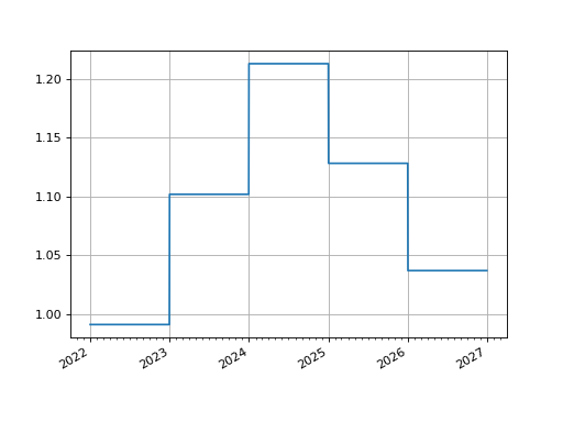
Attributes Summary
Methods Summary
copy()Create an identical copy of the curve object.
csolve()Solves and sets the coefficients,
c, of thePPSpline.from_json(curve, **kwargs)Reconstitute a curve from JSON.
plot(tenor[, right, left, comparators, ...])Plot given forward tenor rates from the curve.
rate(effective, termination[, modifier, ...])Calculate the rate on the Curve using DFs.
roll(tenor)Create a new curve with its shape translated in time but an identical initial node date.
shift(spread[, id, composite, collateral])Create a new curve by vertically adjusting the curve by a set number of basis points.
to_json()Convert the parameters of the curve to JSON format.
translate(start[, t])Create a new curve with an initial node date moved forward keeping all else constant.
Attributes Documentation
- collateral = None#
Methods Documentation
- csolve()#
Solves and sets the coefficients,
c, of thePPSpline.- Return type:
None
Notes
Only impacts curves which have a knot sequence,
t, and aPPSpline. Only solves ifcnot given at curve initialisation.Uses the
spline_endpointsattribute on the class to determine the solving method.
- classmethod from_json(curve, **kwargs)#
Reconstitute a curve from JSON.
- plot(tenor, right=NoInput.blank, left=NoInput.blank, comparators=[], difference=False, labels=[])#
Plot given forward tenor rates from the curve.
- Parameters:
tenor (str) – The tenor of the forward rates to plot, e.g. “1D”, “3M”.
right (datetime or str, optional) – The right bound of the graph. If given as str should be a tenor format defining a point measured from the initial node date of the curve. Defaults to the final node of the curve minus the
tenor.left (datetime or str, optional) – The left bound of the graph. If given as str should be a tenor format defining a point measured from the initial node date of the curve. Defaults to the initial node of the curve.
comparators (list[Curve]) – A list of curves which to include on the same plot as comparators.
difference (bool) – Whether to plot as comparator minus base curve or outright curve levels in plot. Default is False.
labels (list[str]) – A list of strings associated with the plot and comparators. Must be same length as number of plots.
- Returns:
(fig, ax, line)
- Return type:
Matplotlib.Figure, Matplotplib.Axes, Matplotlib.Lines2D
- rate(effective, termination, modifier=NoInput.blank, float_spread=None, spread_compound_method=None)#
Calculate the rate on the Curve using DFs.
If rates are sought for dates prior to the initial node of the curve None will be returned.
- Parameters:
effective (datetime) – The start date of the period for which to calculate the rate.
termination (datetime or str) – The end date of the period for which to calculate the rate.
modifier (str, optional) – The day rule if determining the termination from tenor. If False is determined from the Curve modifier.
float_spread (float, optional) – A float spread can be added to the rate in certain cases.
spread_compound_method (str in {"none_simple", "isda_compounding"}) – The method if adding a float spread. If “none_simple” is used this results in an exact calculation. If “isda_compounding” or “isda_flat_compounding” is used this results in an approximation.
- Return type:
Notes
Calculating rates from a curve implies that the conventions attached to the specific index, e.g. USD SOFR, or GBP SONIA, are applicable and these should be set at initialisation of the
Curve. Thus, the convention used to calculate therateis taken from theCurvefrom whichrateis called.modifieris only used if a tenor is given as the termination.Major indexes, such as legacy IBORs, and modern RFRs typically use a
conventionwhich is either “Act365F” or “Act360”. These conventions do not need additional parameters, such as the termination of a leg, the frequency or a leg or whether it is a stub to calculate a DCF.Adding Floating Spreads
An optimised method for adding floating spreads to a curve rate is provided. This is quite restrictive and mainly used internally to facilitate other parts of the library.
When
spread_compound_methodis “none_simple” the spread is a simple linear addition.When using “isda_compounding” or “isda_flat_compounding” the curve is assumed to be comprised of RFR rates and an approximation is used to derive to total rate.
Examples
In [1]: curve_act365f = Curve(
   ...:     nodes={
   ...:         dt(2022, 1, 1): 1.0,
   ...:         dt(2022, 2, 1): 0.98,
   ...:         dt(2022, 3, 1): 0.978,
   ...:     },
   ...:     convention='Act365F'
   ...: )
   ...:

In [2]: curve_act365f.rate(dt(2022, 2, 1), dt(2022, 3, 1))
Out[2]: 2.6657902424774402
Using a different convention will result in a different rate:
In [3]: curve_act360 = Curve(
   ...:     nodes={
   ...:         dt(2022, 1, 1): 1.0,
   ...:         dt(2022, 2, 1): 0.98,
   ...:         dt(2022, 3, 1): 0.978,
   ...:     },
   ...:     convention='Act360'
   ...: )
   ...:

In [4]: curve_act360.rate(dt(2022, 2, 1), dt(2022, 3, 1))
Out[4]: 2.6292725679229547
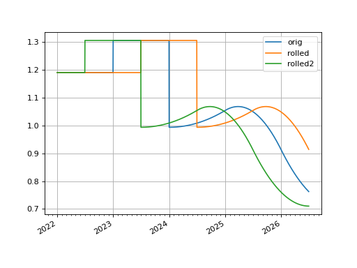
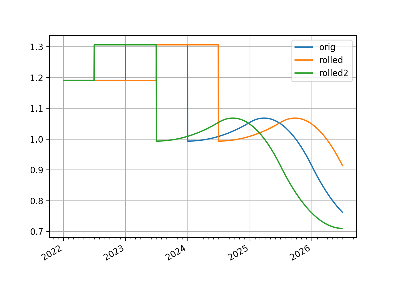
- roll(tenor)#
Create a new curve with its shape translated in time but an identical initial node date.
This curve adjustment is a simulation of a future state of the market where forward rates are assumed to have moved so that the present day’s curve shape is reflected in the future (or the past). This is often used in trade strategy analysis.
- Parameters:
tenor (datetime or str) – The date or tenor by which to roll the curve. If a tenor, as str, will derive the datetime as measured from the initial node date. If supplying a negative tenor, or a past datetime, there is a limit to how far back the curve can be rolled - it will first roll backwards and then attempt to
translate()forward to maintain the initial node date.- Return type:
Examples
The basic use of this function translates a curve forward in time and the plot demonstrates its rates are exactly the same as initially forecast.
In [1]: curve = Curve(
   ...:     nodes = {
   ...:         dt(2022, 1, 1): 1.0,
   ...:         dt(2023, 1, 1): 0.988,
   ...:         dt(2024, 1, 1): 0.975,
   ...:         dt(2025, 1, 1): 0.965,
   ...:         dt(2026, 1, 1): 0.955,
   ...:         dt(2027, 1, 1): 0.9475
   ...:     },
   ...:     t = [
   ...:         dt(2024, 1, 1), dt(2024, 1, 1), dt(2024, 1, 1), dt(2024, 1, 1),
   ...:         dt(2025, 1, 1),
   ...:         dt(2026, 1, 1),
   ...:         dt(2027, 1, 1), dt(2027, 1, 1), dt(2027, 1, 1), dt(2027, 1, 1),
   ...:     ],
   ...: )
   ...:

In [2]: rolled_curve = curve.roll("6m")

In [3]: rolled_curve2 = curve.roll("-6m")

In [4]: curve.plot(
   ...:     "1d",
   ...:     comparators=[rolled_curve, rolled_curve2],
   ...:     labels=["orig", "rolled", "rolled2"],
   ...:     right=dt(2026, 7, 1),
   ...: )
   ...:
Out[4]:
(<Figure size 640x480 with 1 Axes>,
 <Axes: >,
 [<matplotlib.lines.Line2D at 0x7f0aa7e66750>,
  <matplotlib.lines.Line2D at 0x7f0aac13d690>,
  <matplotlib.lines.Line2D at 0x7f0aac13fb90>])
(
Source code,png,hires.png,pdf)
- shift(spread, id=None, composite=True, collateral=None)#
Create a new curve by vertically adjusting the curve by a set number of basis points.
This curve adjustment preserves the shape of the curve but moves it up or down as a translation. This method is suitable as a way to assess value changes of instruments when a parallel move higher or lower in yields is predicted.
- Parameters:
spread (float, Dual, Dual2) – The number of basis points added to the existing curve.
id (str, optional) – Set the id of the returned curve.
composite (bool, optional) – If True will return a CompositeCurve that adds a flat curve to the existing curve. This results in slower calculations but the curve will maintain a dynamic association with the underlying curve and will change if the underlying curve changes.
collateral (str, optional) – Designate a collateral tag for the curve which is used by other methods.
- Return type:
Examples
In [1]: from rateslib.curves import Curve
In [2]: curve = Curve(
   ...:     nodes = {
   ...:         dt(2022, 1, 1): 1.0,
   ...:         dt(2023, 1, 1): 0.988,
   ...:         dt(2024, 1, 1): 0.975,
   ...:         dt(2025, 1, 1): 0.965,
   ...:         dt(2026, 1, 1): 0.955,
   ...:         dt(2027, 1, 1): 0.9475
   ...:     },
   ...:     t = [
   ...:         dt(2024, 1, 1), dt(2024, 1, 1), dt(2024, 1, 1), dt(2024, 1, 1),
   ...:         dt(2025, 1, 1),
   ...:         dt(2026, 1, 1),
   ...:         dt(2027, 1, 1), dt(2027, 1, 1), dt(2027, 1, 1), dt(2027, 1, 1),
   ...:     ],
   ...: )
   ...:

In [3]: shifted_curve = curve.shift(25)

In [4]: curve.plot("1d", comparators=[shifted_curve], labels=["orig", "shift"])
Out[4]:
(<Figure size 640x480 with 1 Axes>,
 <Axes: >,
 [<matplotlib.lines.Line2D at 0x7f0aa5c36750>,
  <matplotlib.lines.Line2D at 0x7f0aa5cd8810>])
(
Source code,png,hires.png,pdf)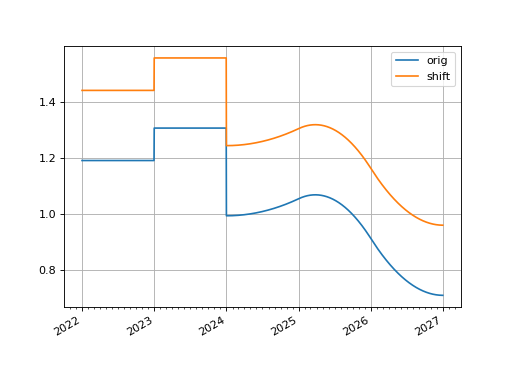
- to_json()#
Convert the parameters of the curve to JSON format.
- Return type:
str
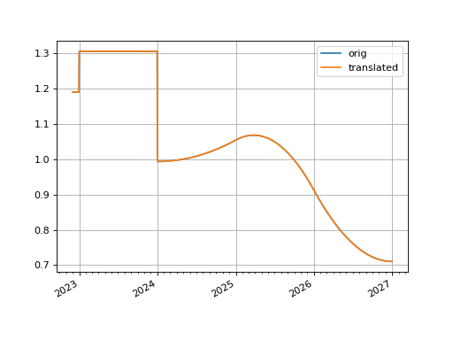
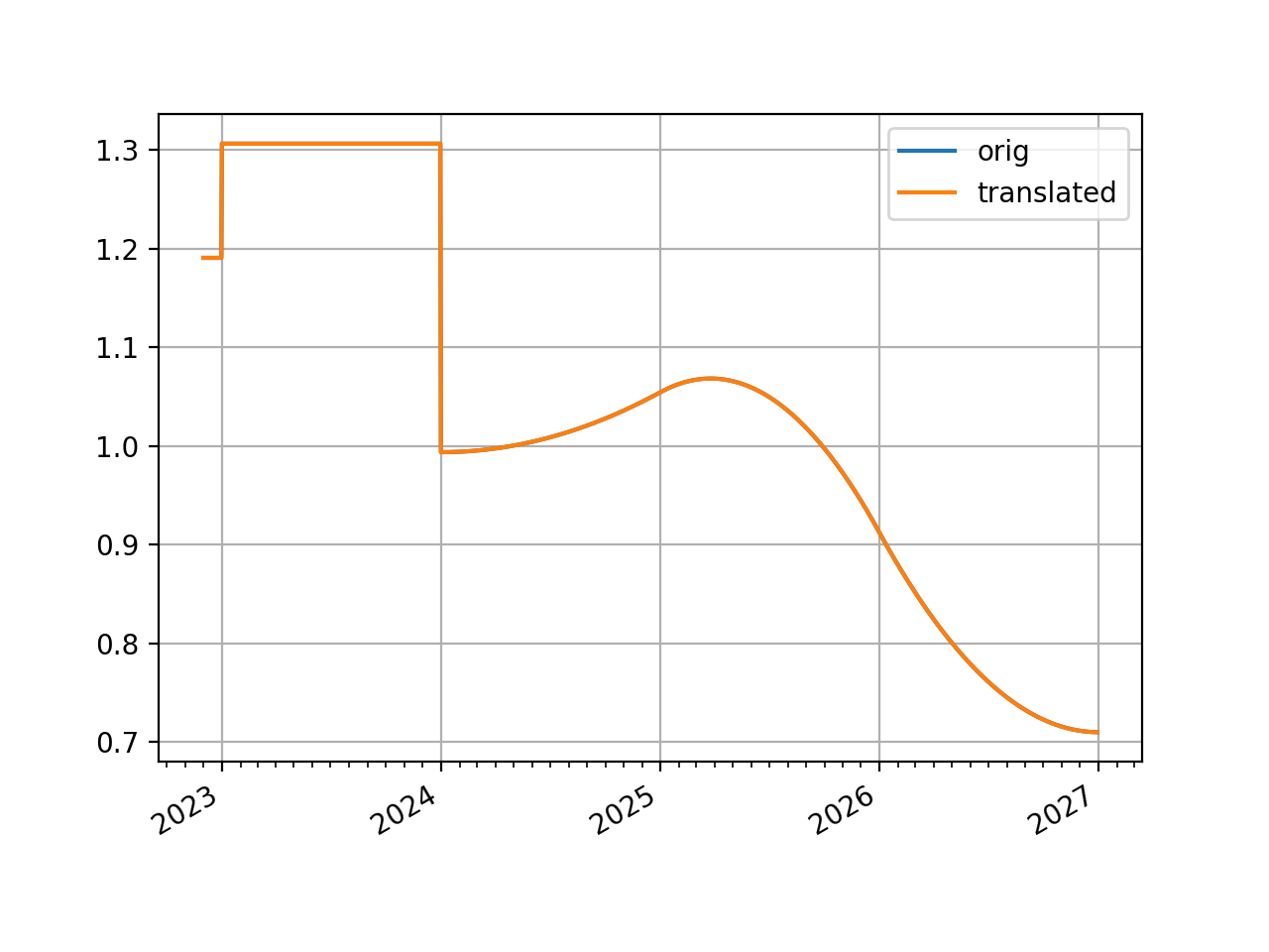
- translate(start, t=False)#
Create a new curve with an initial node date moved forward keeping all else constant.
This curve adjustment preserves forward curve expectations as time evolves. This method is suitable as a way to create a subsequent opening curve from a previous day’s closing curve.
- Parameters:
start (datetime) – The new initial node date for the curve, must be in the domain: (node_date[0], node_date[1]]
t (bool) – Set to True if the initial knots of the knot sequence should be translated forward.
- Return type:
Examples
The basic use of this function translates a curve forward in time and the plot demonstrates its rates are exactly the same as initially forecast.
In [1]: curve = Curve(
   ...:     nodes = {
   ...:         dt(2022, 1, 1): 1.0,
   ...:         dt(2023, 1, 1): 0.988,
   ...:         dt(2024, 1, 1): 0.975,
   ...:         dt(2025, 1, 1): 0.965,
   ...:         dt(2026, 1, 1): 0.955,
   ...:         dt(2027, 1, 1): 0.9475
   ...:     },
   ...:     t = [
   ...:         dt(2024, 1, 1), dt(2024, 1, 1), dt(2024, 1, 1), dt(2024, 1, 1),
   ...:         dt(2025, 1, 1),
   ...:         dt(2026, 1, 1),
   ...:         dt(2027, 1, 1), dt(2027, 1, 1), dt(2027, 1, 1), dt(2027, 1, 1),
   ...:     ],
   ...: )
   ...:

In [2]: translated_curve = curve.translate(dt(2022, 12, 1))

In [3]: curve.plot(
   ...:     "1d",
   ...:     comparators=[translated_curve],
   ...:     labels=["orig", "translated"],
   ...:     left=dt(2022, 12, 1),
   ...: )
   ...:
Out[3]:
(<Figure size 640x480 with 1 Axes>,
 <Axes: >,
 [<matplotlib.lines.Line2D at 0x7f0aa5aaa6d0>,
  <matplotlib.lines.Line2D at 0x7f0aa4f53c10>])
(
Source code,png,hires.png,pdf)
In [4]: curve.nodes
Out[4]:
{datetime.datetime(2022, 1, 1, 0, 0): 1.0,
 datetime.datetime(2023, 1, 1, 0, 0): 0.988,
 datetime.datetime(2024, 1, 1, 0, 0): 0.975,
 datetime.datetime(2025, 1, 1, 0, 0): 0.965,
 datetime.datetime(2026, 1, 1, 0, 0): 0.955,
 datetime.datetime(2027, 1, 1, 0, 0): 0.9475}

In [5]: translated_curve.nodes
Out[5]:
{datetime.datetime(2022, 12, 1, 0, 0): 1.0,
 datetime.datetime(2023, 1, 1, 0, 0): 0.9989751829682344,
 datetime.datetime(2024, 1, 1, 0, 0): 0.9858307726660208,
 datetime.datetime(2025, 1, 1, 0, 0): 0.9757196878181642,
 datetime.datetime(2026, 1, 1, 0, 0): 0.9656086029703076,
 datetime.datetime(2027, 1, 1, 0, 0): 0.9580252893344151}
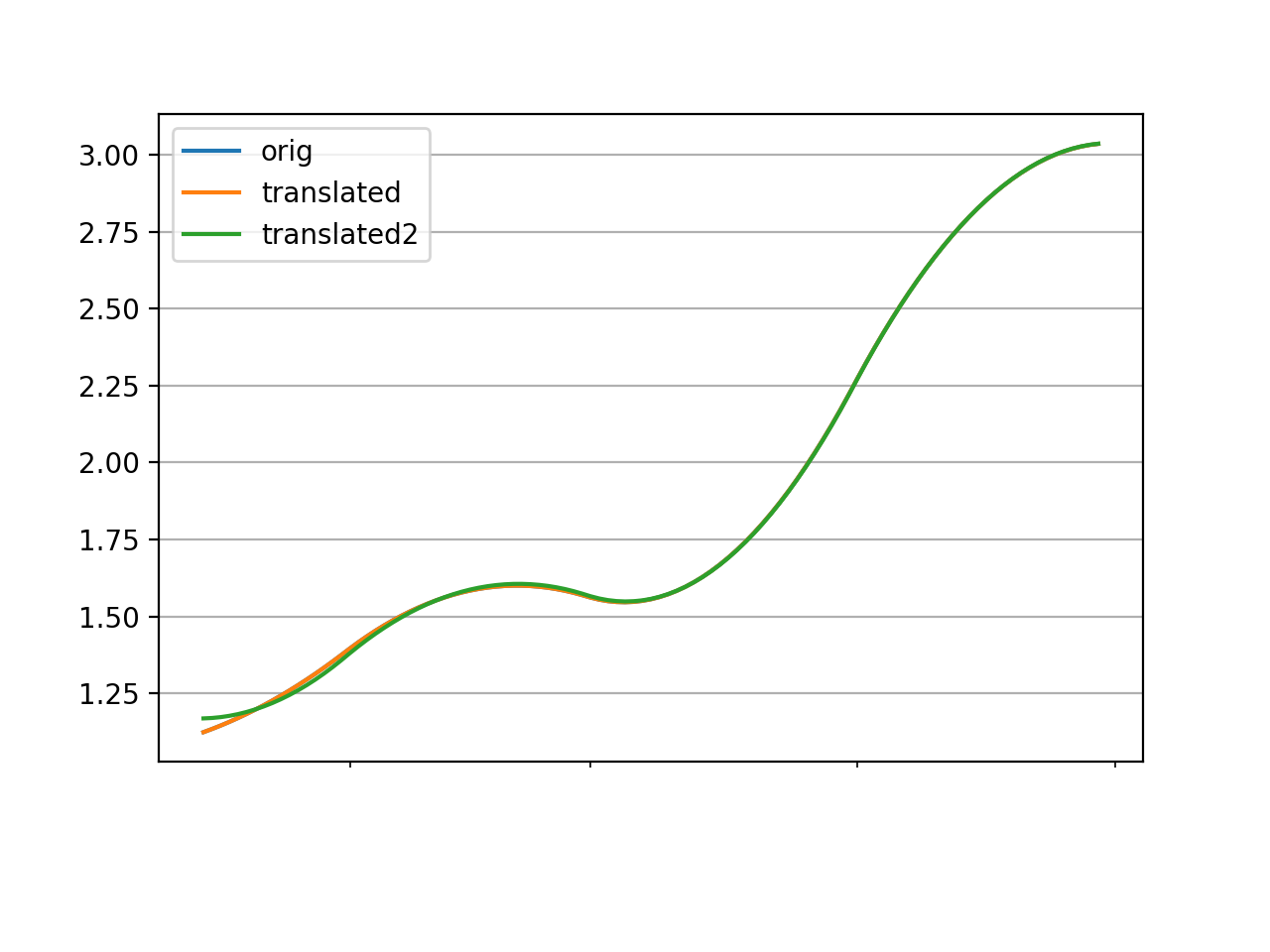
When a curve has a log-cubic spline the knot dates can be preserved or translated with the
targument. Preserving the knot dates preserves the interpolation of the curve. A knot sequence for a mixed curve which begins afterstartwill not be affected in either case.In [6]: curve = Curve( ...: nodes={ ...: dt(2022, 1, 1): 1.0, ...: dt(2022, 2, 1): 0.999, ...: dt(2022, 3, 1): 0.9978, ...: dt(2022, 4, 1): 0.9963, ...: dt(2022, 5, 1): 0.9940 ...: }, ...: t = [dt(2022, 1, 1), dt(2022, 1, 1), dt(2022, 1, 1), dt(2022, 1, 1), ...: dt(2022, 2, 1), dt(2022, 3, 1), dt(2022, 4, 1), ...: dt(2022, 5, 1), dt(2022, 5, 1), dt(2022, 5, 1), dt(2022, 5, 1)] ...: ) ...: In [7]: translated_curve = curve.translate(dt(2022, 1, 15)) In [8]: translated_curve2 = curve.translate(dt(2022, 1, 15), t=True) In [9]: curve.plot("1d", left=dt(2022, 1, 15), comparators=[translated_curve, translated_curve2], labels=["orig", "translated", "translated2"]) Out[9]: (<Figure size 640x480 with 1 Axes>, <Axes: >, [<matplotlib.lines.Line2D at 0x7f0aa4e29390>, <matplotlib.lines.Line2D at 0x7f0aa4e290d0>, <matplotlib.lines.Line2D at 0x7f0aa4e24710>])
(
Source code,png,hires.png,pdf)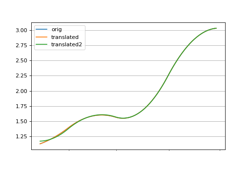