Exploring Bond Basis and Bond Futures DV01#
The first task for example purposes is to create a US-Treasury Instrument, that will serve as the CTD bond, and a CME 10Y Note Future.
In [1]: ust = FixedRateBond(
   ...:     effective=dt(2017, 8, 15),
   ...:     termination=dt(2024, 8, 15),
   ...:     fixed_rate=2.375,
   ...:     notional=-1e6,
   ...:     spec="ust",
   ...:     curves="bcurve",
   ...: )
   ...:

In [2]: usbf = BondFuture(
   ...:     coupon=6.0,
   ...:     delivery=(dt(2017, 12, 1), dt(2017, 12, 29)),
   ...:     basket=[ust],
   ...:     calc_mode="ust_long",
   ...:     nominal=100e3,
   ...:     contracts=10,
   ...: )
   ...:
Without constructing any Curves we can analyse this bond future with static data,
In [3]: df = usbf.dlv(
...: future_price=125.2656,
...: prices=[101.2266],
...: repo_rate=1.499,
...: settlement=dt(2017, 10, 10),
...: delivery=dt(2017, 12, 29),
...: convention="act360",
...: )
...:
In [4]: with option_context("display.float_format", lambda x: '%.6f' % x):
...: print(df)
...:
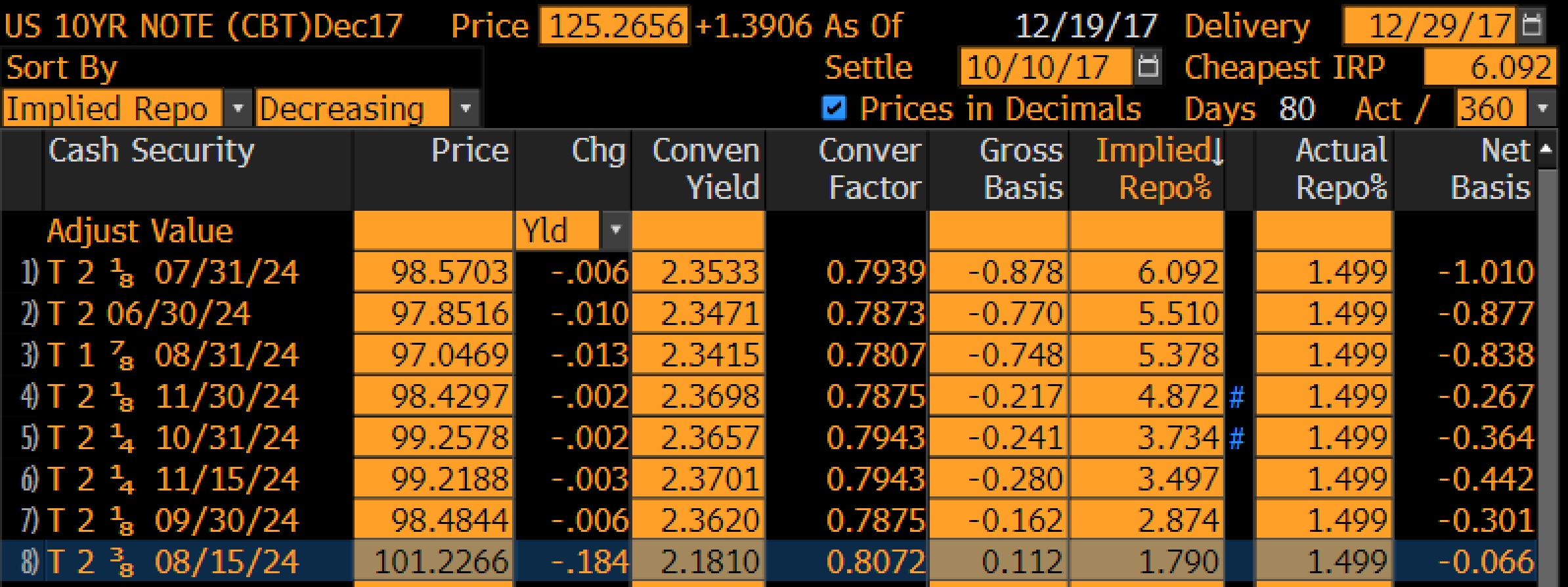
Bond Price YTM C.Factor Gross Basis Implied Repo Actual Repo Net Basis
0 2.375% 15-08-2024 101.226600 2.180980 0.807200 0.112208 1.790009 1.499000 -0.065696
A comparison with Bloomberg is shown below,
Building a curve to reprice the Instruments#
The above calculations are performed with analogue bond formulae. We can build and Solve a Curve.
In [5]: bcurve = Curve(
   ...:     nodes={dt(2017, 10, 9): 1.0, dt(2024, 8, 17): 1.0},
   ...:     calendar="nyc",
   ...:     convention="act360",
   ...:     id="bcurve"
   ...: )
   ...:

In [6]: solver = Solver(
   ...:     curves=[bcurve],
   ...:     instruments=[(ust, (), {"metric": "ytm"})],
   ...:     s=[2.18098],
   ...:     instrument_labels=["bond ytm"],
   ...:     id="bonds",
   ...: )
   ...:
SUCCESS: `func_tol` reached after 5 iterations (levenberg_marquardt), `f_val`: 1.480704752901436e-13, `time`: 0.0150s
The following is a comparison between analogue methods without a Curve and digital methods that use this numerical Curve and discounted cashflows, to measure the risk sensitivity of the bond.
Duration and Convexity
In [7]: ust.duration(
   ...:     ytm=2.18098,
   ...:     settlement=dt(2017, 10, 10),
   ...:     metric="risk"
   ...: ) * -100
   ...:
Out[7]: -637.3286241497959

In [8]: ust.convexity(
   ...:     ytm=2.18098,
   ...:     settlement=dt(2017, 10, 10)
   ...: )
   ...:
Out[8]: 0.45171236667241027
Delta and Gamma
In [9]: ust.delta(solver=solver)
Out[9]:
local_ccy                       usd
display_ccy                     usd
type        solver label
instruments bonds  bond ytm -637.57

In [10]: ust.gamma(solver=solver)
Out[10]:
type                                              instruments
solver                                                  bonds
label                                                bond ytm
local_ccy display_ccy type        solver label
usd       usd         instruments bonds  bond ytm        0.45
Metrics for futures#
We can use the same principle to measure the bond future.
Duration and Convexity
In [11]: usbf.duration(
   ....:     future_price=125.2656,
   ....:     delivery=dt(2017, 12, 29),
   ....:     metric="risk"
   ....: )[0] * -100
   ....:
Out[11]: -765.4459667407934

In [12]: usbf.convexity(
   ....:     future_price=125.2656,
   ....:     delivery=dt(2017, 12, 29),
   ....: )[0]
   ....:
Out[12]: 0.5268864798372334
Delta and Gamma
In [13]: usbf.delta(solver=solver)
Out[13]:
local_ccy                       gbp
display_ccy                     gbp
type        solver label
instruments bonds  bond ytm -765.92

In [14]: usbf.gamma(solver=solver)
Out[14]:
type                                              instruments
solver                                                  bonds
label                                                bond ytm
local_ccy display_ccy type        solver label
gbp       gbp         instruments bonds  bond ytm        0.53
The above Curve and Solver are not completely useful for a bond future, however. An important part of its pricing is the repo rate until delivery, so we extend the Curve and Solver to have this relevant pricing component.
In [15]: bcurve = Curve(
   ....:     nodes={
   ....:         dt(2017, 10, 9): 1.0,
   ....:         dt(2017, 12, 29): 1.0,  #  node for the repo rate to delivery
   ....:         dt(2024, 8, 17): 1.0,
   ....:     },
   ....:     calendar="nyc",
   ....:     convention="act360",
   ....:     id="bcurve",
   ....: )
   ....:

In [16]: solver = Solver(
   ....:     curves=[bcurve],
   ....:     instruments=[
   ....:         IRS(dt(2017, 10, 9), dt(2017, 12, 29), spec="usd_irs", curves="bcurve"),
   ....:         (ust, (), {"metric": "ytm"})
   ....:     ],
   ....:     s=[1.790, 2.18098],
   ....:     instrument_labels=["repo", "bond ytm"],
   ....:     id="bonds",
   ....: )
   ....:
SUCCESS: `func_tol` reached after 5 iterations (levenberg_marquardt), `f_val`: 1.5354470289087182e-13, `time`: 0.0164s
Revised Delta and Gamma including the repo rate
In [17]: usbf.delta(solver=solver)
Out[17]:
local_ccy                       gbp
display_ccy                     gbp
type        solver label
instruments bonds  repo       27.97
                   bond ytm -792.70

In [18]: usbf.gamma(solver=solver)
Out[18]:
type                                              instruments
solver                                                  bonds
label                                                    repo bond ytm
local_ccy display_ccy type        solver label
gbp       gbp         instruments bonds  repo           -0.00    -0.02
                                         bond ytm       -0.02     0.56
Observe that in this construction the exposure to the bond yield-to-maturity is actually close to the analogue DV01 of the future with spot delivery.
In [19]: usbf.duration(
   ....:     future_price=125.2656,
   ....:     delivery=dt(2017, 10, 10),
   ....:     metric="risk"
   ....: )[0] * -100
   ....:
Out[19]: -788.5695839010873
This calculation is the same as the spot DV01 of the CTD bond multiplied by the conversion factor, and in this case the spot CTD DV01 is priced from the given futures price assuming a futures delivery date at spot.