Bond Future CTD Multi-Scenario Analysis#
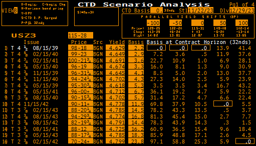
In late 2023 CTD analysis of the US 30Y Treasury Bond Future was worth exploring because quickly rising yields led to multiple changes in the CTD bond.
This page will demonstrate how one might use rateslib to perform some of this analysis.
First we need to configure all of the Instruments and their prices. This is shown statically below (and actually there were many more bonds available in this basket, but this group proved to be the most relevant).
In [1]: data = DataFrame(
...: data= [
...: [FixedRateBond(dt(2022, 1, 1), dt(2039, 8, 15), fixed_rate=4.5, spec="ust", curves="bcurve"), 98.6641],
...: [FixedRateBond(dt(2022, 1, 1), dt(2040, 2, 15), fixed_rate=4.625, spec="ust", curves="bcurve"), 99.8203],
...: [FixedRateBond(dt(2022, 1, 1), dt(2041, 2, 15), fixed_rate=4.75, spec="ust", curves="bcurve"), 100.7734],
...: [FixedRateBond(dt(2022, 1, 1), dt(2040, 5, 15), fixed_rate=4.375, spec="ust", curves="bcurve"), 96.6953],
...: [FixedRateBond(dt(2022, 1, 1), dt(2039, 11, 15), fixed_rate=4.375, spec="ust", curves="bcurve"), 97.0781],
...: [FixedRateBond(dt(2022, 1, 1), dt(2040, 11, 15), fixed_rate=4.25, spec="ust", curves="bcurve"), 94.8516],
...: [FixedRateBond(dt(2022, 1, 1), dt(2039, 5, 15), fixed_rate=4.25, spec="ust", curves="bcurve"), 96.0469],
...: [FixedRateBond(dt(2022, 1, 1), dt(2041, 5, 15), fixed_rate=4.375, spec="ust", curves="bcurve"), 96.1250],
...: [FixedRateBond(dt(2022, 1, 1), dt(2040, 8, 15), fixed_rate=3.875, spec="ust", curves="bcurve"), 90.5938],
...: [FixedRateBond(dt(2022, 1, 1), dt(2042, 11, 15), fixed_rate=4.00, spec="ust", curves="bcurve"), 90.4766],
...: [FixedRateBond(dt(2022, 1, 1), dt(2043, 2, 15), fixed_rate=3.875, spec="ust", curves="bcurve"), 88.7656],
...: [FixedRateBond(dt(2022, 1, 1), dt(2043, 8, 15), fixed_rate=4.375, spec="ust", curves="bcurve"), 95.0703],
...: [FixedRateBond(dt(2022, 1, 1), dt(2042, 8, 15), fixed_rate=3.375, spec="ust", curves="bcurve"), 82.7188],
...: [FixedRateBond(dt(2022, 1, 1), dt(2041, 8, 15), fixed_rate=3.75, spec="ust", curves="bcurve"), 88.4766],
...: [FixedRateBond(dt(2022, 1, 1), dt(2042, 5, 15), fixed_rate=3.25, spec="ust", curves="bcurve"), 81.3828],
...: [FixedRateBond(dt(2022, 1, 1), dt(2039, 2, 15), fixed_rate=3.50, spec="ust", curves="bcurve"), 88.1406],
...: ],
...: columns=["bonds", "prices"],
...: )
...:
In [2]: usz3 = BondFuture( # Construct the BondFuture Instrument
...: coupon=6.0,
...: delivery=(dt(2023, 12, 1), dt(2023, 12, 29)),
...: basket=data["bonds"],
...: nominal=100e3,
...: calendar="nyc",
...: currency="usd",
...: calc_mode="ust_long",
...: )
...:
In [3]: dlv = usz3.dlv( # Analyse the deliverables as of the current prices
...: future_price=115.9688,
...: prices=data["prices"],
...: settlement=dt(2023, 11, 22),
...: repo_rate=5.413,
...: convention="act360",
...: )
...:
In [4]: with option_context("display.float_format", lambda x: '%.6f' % x):
...: print(dlv)
...:
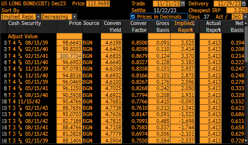
Bond Price YTM C.Factor Gross Basis Implied Repo Actual Repo Net Basis
0 4.500% 15-08-2039 98.664100 4.619845 0.850000 0.090620 3.524883 5.413000 0.193813
1 4.625% 15-02-2040 99.820300 4.640299 0.859800 0.110326 3.414667 5.413000 0.207571
2 4.750% 15-02-2041 100.773400 4.683516 0.867900 0.124078 3.370355 5.413000 0.214245
3 4.375% 15-05-2040 96.695300 4.664509 0.832700 0.128080 3.183256 5.413000 0.221788
4 4.375% 15-11-2039 97.078100 4.635787 0.835800 0.151377 2.937423 5.413000 0.247214
5 4.250% 15-11-2040 94.851600 4.693166 0.816600 0.151478 2.875131 5.413000 0.247621
6 4.250% 15-05-2039 96.046900 4.609951 0.826700 0.175493 2.596310 5.413000 0.278286
7 4.375% 15-05-2041 96.125000 4.702505 0.826800 0.241996 2.050082 5.413000 0.332531
8 3.875% 15-08-2040 90.593800 4.692225 0.779400 0.207717 1.931253 5.413000 0.327917
9 4.000% 15-11-2042 90.476600 4.768069 0.776600 0.415230 -0.092797 5.413000 0.512418
10 3.875% 15-02-2043 88.765600 4.773830 0.761000 0.513343 -1.340559 5.413000 0.623372
11 4.375% 15-08-2043 95.070300 4.762610 0.814700 0.590519 -1.522844 5.413000 0.686099
12 3.375% 15-08-2042 82.718800 4.781496 0.709100 0.485324 -1.698548 5.413000 0.611235
13 3.750% 15-08-2041 88.476600 4.715795 0.758300 0.537459 -1.744253 5.413000 0.658261
14 3.250% 15-05-2042 81.382800 4.777948 0.697400 0.506159 -2.100187 5.413000 0.628911
15 3.500% 15-02-2039 88.140600 4.590394 0.755000 0.584156 -2.536722 5.413000 0.727850
Compared with the Bloomberg read out for the same data:
Analysing the CTD on Parallel Yield Changes#
In order to analyse what happens to bond prices under a parallel shift of the yield curve it is
more accurate to calculate a discount factor Curve and use the
shift() method to ensure this is consistently applied to every Bond.
This Curve has a node date placed at the maturity of every bond so that we will be able to
reprice every Bond price exactly when using a Solver.
In [5]: unsorted_nodes = {
   ...:     dt(2023, 11, 21): 1.0, #  Today's date
   ...:     **{_.leg1.schedule.termination: 1.0 for _ in data["bonds"]}
   ...: }
   ...:

In [6]: bcurve = Curve(
   ...:     nodes=dict(sorted(unsorted_nodes.items(), key=lambda _: _[0])),
   ...:     id="bcurve",
   ...: )
   ...:

In [7]: solver = Solver(
   ...:     curves=[bcurve],
   ...:     instruments=data["bonds"],
   ...:     s=data["prices"],
   ...: )
   ...:
SUCCESS: `func_tol` reached after 4 iterations (levenberg_marquardt), `f_val`: 2.1530976153446382e-17, `time`: 0.2155s
It is now possible to calculate any bond price under a shifted curve. Consider,
In [8]: data["bonds"][0].rate(curves=bcurve.shift(10))  # price of 4.5% Aug '39 with +10bps in rates.
Out[8]: <Dual: 97.546189, (bcurve0, bcurve1, bcurve2, ...), [-71.2, 44.4, -0.0, ...]>
Note
Once a Solver has been used the Curve contains 1st order AD information (usually for risk sensitivity calculations). For the processes we will be performing below this is not necessary and it makes for faster calculations to turn it off.
In [9]: bcurve._set_ad_order(order=0)

In [10]: data["bonds"][0].rate(curves=bcurve.shift(10))
Out[10]: 97.5461891863331
Calculating the DV01 of the BondFuture#
The ‘risk’ DV01 of the BondFuture is calculated by:
implying the invoice price of each Bond in the basket from the BondFuture price,
determining each of those Bonds ‘risk’ duration for settlement at delivery, with that invoice price, and then dividing by the conversion factor,
selecting the result that coincides with the CTD.
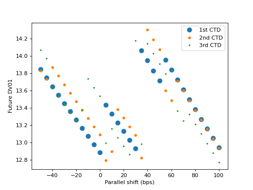
We will aim to plot a graph of BondFuture DV01s versus parallel shifts in the curve. Since the Bonds are, in some cases, very similar from a CTD perspective we will plot the CTD bond, and the second and third CTD bonds.
In [11]: x, y1, y2, y3 = [], [], [], []  # containers for graph data

In [12]: for shift in range(-50, 105, 5):
   ....:     scurve = bcurve.shift(shift)                   # Shift the curve by a number of bps
   ....:     future_price = usz3.rate(curves=scurve)        # Find the future's price from the curve
   ....:     ctd_indexes = usz3.ctd_index(                  # Determine the CTDs with new prices
   ....:         future_price=future_price,
   ....:         prices=[_.rate(curves=scurve) for _ in data["bonds"]],
   ....:         settlement=dt(2023, 11, 22),
   ....:         ordered=True,
   ....:     )
   ....:     risks = usz3.duration(future_price)            # Find the Future DV01 from each Bond in basket
   ....:     y1.append(risks[ctd_indexes[0]])
   ....:     y2.append(risks[ctd_indexes[1]])
   ....:     y3.append(risks[ctd_indexes[2]])
   ....:     x.append(shift)                                # Fill graph containers with data
   ....:
With all the data calculated we can plot the graph.
In [13]: fig, axs = plt.subplots(1,1);

In [14]: axs.plot(x, y1, 'o', markersize=8.0, label="1st CTD");

In [15]: axs.plot(x, y2, 'o', markersize=4.0, label="2nd CTD");

In [16]: axs.plot(x, y3, 'o', markersize=2.0, label="3rd CTD");

In [17]: axs.legend();

In [18]: axs.set_xlabel("Parallel shift (bps)");

In [19]: axs.set_ylabel("Future DV01");
(Source code, png, hires.png, pdf)
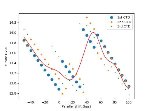
Weighting the Future DV01#
At this stage, calculating the option adjusted DV01 is a probabilistic problem. One that depends upon volatility, time to delivery and the correlation between all of the different bonds.
As a rather egregious approximation we can use a PPSplineF64 to interpolate
(in a least squares sense) over these data points. The knot points of this splines and which
bonds are included (and what weights they could be potentially be assigned in a weighted least
squares calculation) proxies the above mentioned probabilistic variables.
In [20]: pps = PPSplineF64(
   ....:     k=4,
   ....:     t=[-50, -50, -50, -50, -35, -20, 0, 20, 35, 50, 65, 80, 100, 100, 100, 100]
   ....: );
   ....:

In [21]: pps.csolve(x + x + x, y1 + y2 + y3, 0, 0, allow_lsq=True);

In [22]: x2 = [float(_) for _ in range(-50, 101, 1)];

In [23]: axs.plot(x2, pps.ppev(np.array(x2)));
(Source code, png, hires.png, pdf)
Using CMS (CTD Multi-Security) Analysis#
The above analysis can be replicated with the cms() method.
This method replicates the above process for a sequence of provide parallel shifts.
In [24]: usz3.cms(
   ....:     prices=data["prices"],
   ....:     settlement=dt(2023, 11, 22),
   ....:     shifts=[-100, -50, 0, 50, 100]
   ....: )
   ....:
SUCCESS: `func_tol` reached after 4 iterations (levenberg_marquardt), `f_val`: 2.1530976153446382e-17, `time`: 0.2158s
Out[24]:
                 Bond  -100  -50     0   50  100
0   4.500% 15-08-2039  0.00 0.00 -0.00 0.43 1.24
1   4.625% 15-02-2040  0.22 0.11  0.01 0.36 1.12
2   4.750% 15-02-2041  0.69 0.33  0.02 0.20 0.81
3   4.375% 15-05-2040  0.50 0.25  0.03 0.27 0.91
4   4.375% 15-11-2039  0.26 0.15  0.06 0.40 1.13
5   4.250% 15-11-2040  0.84 0.42  0.06 0.17 0.69
6   4.250% 15-05-2039  0.09 0.09  0.09 0.50 1.29
7   4.375% 15-05-2041  1.13 0.60  0.14 0.18 0.64
8   3.875% 15-08-2040  0.99 0.54  0.15 0.20 0.65
9   4.000% 15-11-2042  2.20 1.19  0.34 0.00 0.13
10  3.875% 15-02-2043  2.49 1.39  0.45 0.03 0.09
11  4.375% 15-08-2043  2.59 1.46  0.50 0.11 0.22
12  3.375% 15-08-2042  2.47 1.38  0.45 0.01 0.00
13  3.750% 15-08-2041  1.92 1.15  0.48 0.29 0.53
14  3.250% 15-05-2042  2.44 1.38  0.47 0.04 0.03
15  3.500% 15-02-2039  0.88 0.71  0.56 0.79 1.37
This can be broadly compared with Bloomberg, except this page re-ordered some of the bonds, and is expressed in 32nds instead of decimals above.