FX Forward Rates#
Basic spot FXRates are extended using discount factor based
Curve s to derive
arbitrage free forward FX rates. The basic FXForwards class is
summarised below,
|
Class for storing and calculating FX forward rates. |
|
Return the fx forward rate for a currency pair. |
|
Return the FXSwap mid-market rate for the given currency pair. |
|
Return a cash collateral curve. |
|
Plot given forward FX rates. |
|
Convert an amount of a domestic currency, as of a settlement date into a foreign currency, valued on another date. |
Convert an input of currency cash positions into a single base currency value. |
|
|
Convert a base value with FX rate sensitivities into an array of cash positions by settlement date. |
Introduction#
When calculating forward FX rates the following information is required;
The spot or immediate FX rate observable in the interbank market.
The interest rates in each currency to derive an interest rate parity expression.
The supply and demand factor, that impacts market FX swap or cross-currency swap price dynamics.
Thus the FXForwards class requires this information for
instantiation. The fx_rates argument is available to supply the first item.
The fx_curves argument requires a dict of labelled curves. This has a specific
structure where each curve is labelled as a cash-collateral curve. The first 3 digits
represent the currency of the cashflow and the latter 3 represent the currency in which
that cashflow is collateralized.
Just for the first example, if we suppose that the third element (the supply and demand factor from tenor cross-currency markets) is missing or is zero, then we can instantiate the class with information from only the first two elements.
# This is the spot FX exchange rates
In [1]: fx_rates = FXRates({"eurusd": 1.05}, settlement=dt(2022, 1, 3), base="usd")

# These are the interest rate curves in EUR and USD
In [2]: usd_curve = Curve({dt(2022, 1, 1): 1.0, dt(2023, 1, 1): 0.965})

In [3]: eur_curve = Curve({dt(2022, 1, 1): 1.0, dt(2023, 1, 1): 0.985})

In [4]: fx_curves = {
   ...:     "usdusd": usd_curve,
   ...:     "eureur": eur_curve,
   ...:     "eurusd": eur_curve,  #  <- This is the same as "eureur" since no third factor
   ...: }
   ...:

In [5]: fxf = FXForwards(fx_rates, fx_curves)
With the class instantiated we can use it to calculate forward FX rates.
In [6]: fxf.rate("eurusd", dt(2022, 9,15))
Out[6]: <Dual: 1.065156, (fx_eurusd), [1.0]>
To explicitly verify this we can make this calculation manually with the FX interest rate parity formula. The relevant interest rates are extracted from the curves.
In [7]: usd_curve.rate(dt(2022, 1, 3), dt(2022, 9, 15))
Out[7]: 3.558009544354078

In [8]: eur_curve.rate(dt(2022, 1, 3), dt(2022, 9, 15))
Out[8]: 1.4985577628087257

In [9]: dcf(dt(2022, 1, 3), dt(2022, 9, 15), "act360")
Out[9]: 0.7083333333333334
Cross-Currency Swap and FX Swap Basis#
In this example we will expand the above by adding the third component. Suppose that:
The FX rates are:
EURUSD: 1.05,
GBPUSD: 1.20,
The interest rates are:
USD: 3.5%,
EUR: 1.5%,
GBP: 2.0%,
The cross-currency basis swap rates are:
EUR/USD: -20bps,
GBP/USD: -30bps,
The following configuration gives an approximate representation of this market.
In [10]: fxr = FXRates({"eurusd": 1.05, "gbpusd": 1.20}, settlement = dt(2022, 1, 3))

In [11]: fxf = FXForwards(fxr, {
   ....:     "usdusd": Curve({dt(2022, 1, 1): 1.0, dt(2023, 1, 1): 0.965}, id="uu"),
   ....:     "eureur": Curve({dt(2022, 1, 1): 1.0, dt(2023, 1, 1): 0.985}, id="ee"),
   ....:     "eurusd": Curve({dt(2022, 1, 1): 1.0, dt(2023, 1, 1): 0.987}, id="eu"),
   ....:     "gbpgbp": Curve({dt(2022, 1, 1): 1.0, dt(2023, 1, 1): 0.970}),
   ....:     "gbpusd": Curve({dt(2022, 1, 1): 1.0, dt(2023, 1, 1): 0.973})
   ....: })
   ....:
If we compare this to the above section the forward FX rates for EURUSD is slightly different now that the third component is accounted for with an amended “eurusd” discount curve.
In [12]: fxf.rate("eurusd", dt(2022, 9, 15))
Out[12]: <Dual: 1.066667, (fx_gbpusd, fx_eurusd), [0.0, 1.0]>
We can repeat the above manual calculation with the necessary adjustments.
In [13]: fxf.fx_curves["eurusd"].rate(dt(2022, 1, 3), dt(2022, 9, 15))
Out[13]: 1.2965161483992789
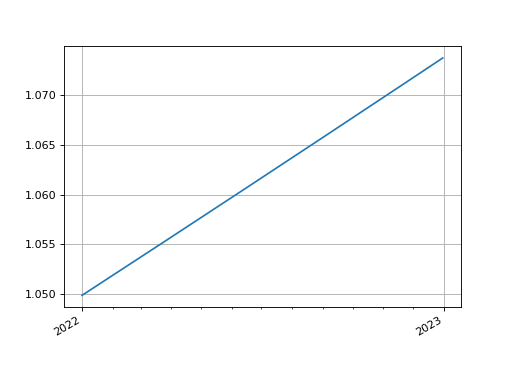
Visualization#
The plot() method exists for the
FXForwards class. We can plot the EURUSD
forward FX rates. Since our curves only contain one flat rate the FX forward rate
reflects a straight upward line when plotted for all settlement dates in the window.
In [14]: fxf.plot("eurusd")
Out[14]:
(<Figure size 640x480 with 1 Axes>,
 <Axes: >,
 [<matplotlib.lines.Line2D at 0x7f0a9ef6c6d0>])
(Source code, png, hires.png, pdf)
ProxyCurves and Discounting#
In a multi-currency framework there are often many intrinsic discount curves that can
be constructed that are not necessary for the initial construction of the
FXForwards class. For example, in the above sections,
the discount curve for
GBP cashflows discounted under a EUR collateral CSA (credit support annex),
the “gbpeur” curve is
not provided at initialisation, nor is the “eurgbp” curve.
In these circumstances the curve() method will derive the
combination of existing curves that can be combined to yield required DFs on-the-fly.
This creates a ProxyCurve.
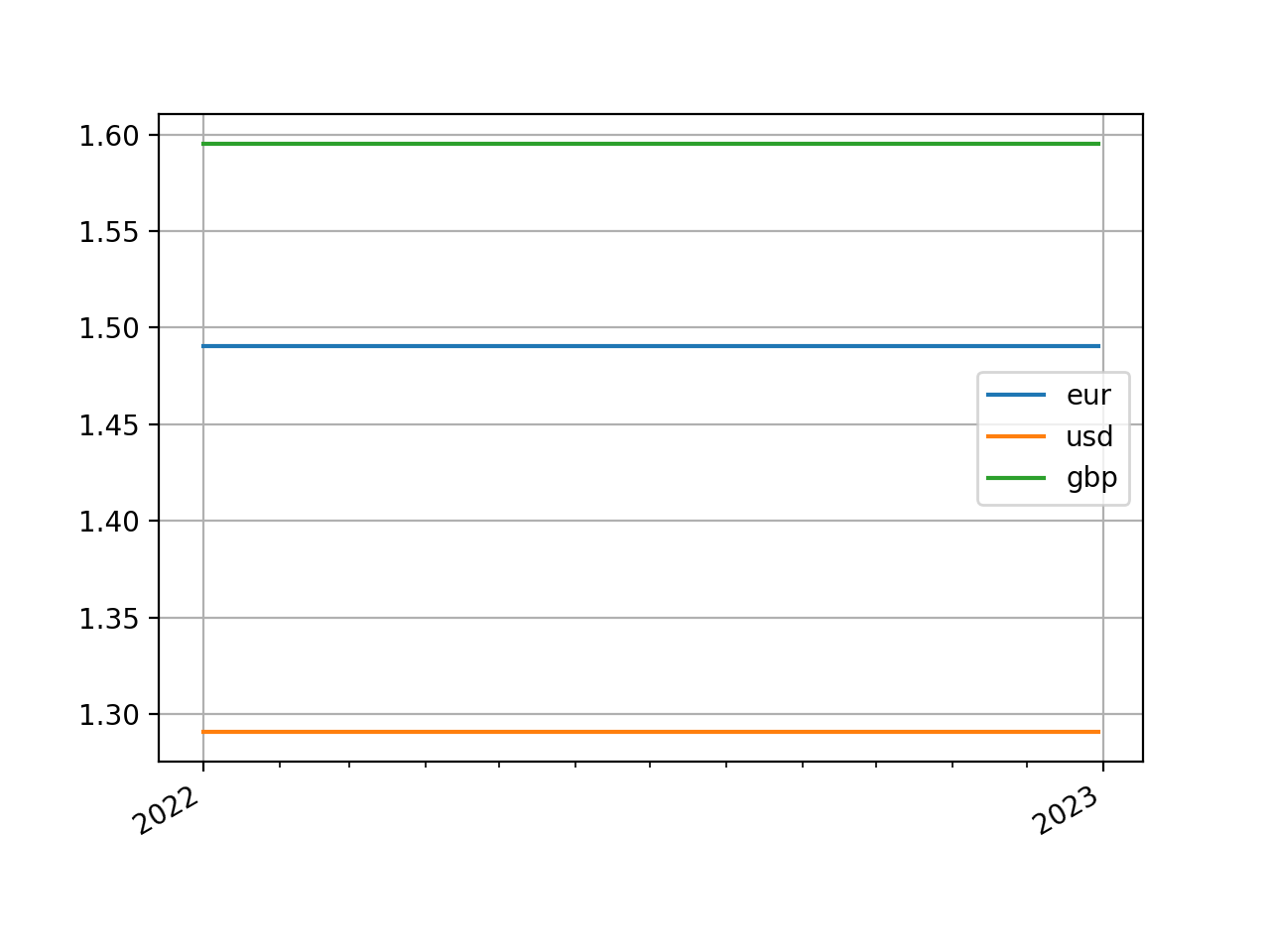
In the above framework GBP is the cheapest to deliver collateral, and USD is the most expensive. We can observe this by calculating the curves in any cash currency for all collateral currencies and plotting. This is demonstrated below.
In [15]: type(fxf.curve("eur", "eur"))
Out[15]: rateslib.curves.Curve

In [16]: type(fxf.curve("eur", "usd"))
Out[16]: rateslib.curves.Curve

In [17]: type(fxf.curve("eur", "gbp"))
Out[17]: rateslib.curves.ProxyCurve

In [18]: fxf.curve("eur", "eur").plot(
   ....:     "1d",
   ....:     labels=["eur", "usd", "gbp"],
   ....:     comparators=[
   ....:         fxf.curve("eur", "usd"),
   ....:         fxf.curve("eur", "gbp")
   ....:     ]
   ....: )
   ....:
Out[18]:
(<Figure size 640x480 with 1 Axes>,
 <Axes: >,
 [<matplotlib.lines.Line2D at 0x7f0a9ed09390>,
  <matplotlib.lines.Line2D at 0x7f0a9ed090d0>,
  <matplotlib.lines.Line2D at 0x7f0a9ecc5b90>])
(Source code, png, hires.png, pdf)

Sensitivity Management#
The FXForwards class functions similarly to the
FXRates class in a sensitivity respect. The same
convert(), positions() and
convert_positions() methods exist to transition between
different representations of cash positions and Dual values.
Since FXForwards are time sensitive the representation of
cashflows on specific dates is important. In the below example the EURUSD rate settles
spot (T+2), and the curves are constructed from the immediate date. FX sensitivity is
then correctly interpreted as opposite currency cashflows on the appropriate
settlement date, whereas the fundamental base value is an NPV and is recorded as an
immediate cash position.
In [19]: positions = fxf.positions(1000, base="usd")

In [20]: positions
Out[20]:
     2022-01-01  2022-01-03
eur        0.00        0.00
gbp        0.00        0.00
usd     1000.00        0.00
In [21]: positions = fxf.positions(Dual(1000, ["fx_eurusd"], [1000]), base="usd")

In [22]: positions
Out[22]:
     2022-01-01  2022-01-03
eur        0.00     1000.00
gbp        0.00        0.00
usd     1000.00    -1050.00
Provided a one-to-one correspondence exists, the positions can be accurately converted into a base value with dual sensitivities.
In [23]: fxf.convert_positions(positions, base="usd")
Out[23]: <Dual: 1000.000000, (fx_gbpusd, fx_eurusd), [0.0, 1000.0]>
It is also possible to take a single cashflow and convert it into another value as of another date.
In [24]: fxf.convert(1000, "usd", "eur", dt(2022, 1, 1), dt(2022, 1, 25))
Out[24]: <Dual: 953.318477, (fx_gbpusd, fx_eurusd), [-0.0, -907.9]>
This cashflow does not demonstrate any sensitivity to interest rates even though
a forward value ought to. This is because the interest rate curves that are
associated with the FXForwards instance are not configured
with automatic differentiation. We can manually instruct this here (only for
purposes of example) and see the
impact, but note use of this private method is not recommended and is usually called
only internally.
In [25]: fxf._set_ad_order(1)

In [26]: fxf.convert(1000, "usd", "eur", dt(2022, 1, 1), dt(2022, 1, 25))
Out[26]: <Dual: 953.318477, (fx_gbpusd, fx_eurusd, eu1, ...), [0.0, -907.9, -63.5, ...]>