How to Handle Turns in Rateslib#

Turns are an artifact present on interest rate curves that reflect a genuine economic effect. To an outsider these often look like discontinuities, outliers, or erroneous data. But, they are an accurate reflection of reality, and should always be included.

The following image is an example of an index, the Riksbank’s SWESTR, which is impacted to an excessive degree by the government’s fiscal policy of applying taxes and fees based on the size of a Swedish bank’s liabilities at year end. In order to either shrink its liabilities or accrue an amount from a depositor that covers the fee, a Swedish bank adjusts its overnight deposit rate for this one day of the year. Because of the scale, any daily variation of regular amplitude at around 2.30%-2.31% is not visible and the curve appears completely flat, but it is not. Data is available on the Riksbank’s website.

SWESTR data showing an egregious end of year turn.

These present challenges when constructing curves, however. Consider the following Curve, which from 1st Dec ‘22 to 31st Jan ‘23 is a flat curve with overnight rates at 1%.

In [1]: curve = Curve({dt(2022, 12, 1): 1.0, dt(2023, 1, 31): 1.0}, id="v")

In [2]: solver = Solver(
   ...:     curves=[curve],
   ...:     instruments=[IRS(dt(2022, 12, 1), "1b", "A", curves=curve)],
   ...:     s=[1.0],
   ...: )
   ...: 
SUCCESS: `func_tol` reached after 2 iterations (levenberg_marquardt), `f_val`: 6.938680060733138e-16, `time`: 0.0010s

For the next part, when we add a turn, we will compare back to this curve. So, for the record, three relevant discount factors (DFs) on it are:

In [3]: curve[dt(2022, 12, 31)]
Out[3]: <Dual: 0.999178, (v0, v1), [0.5, 0.5]>

In [4]: curve[dt(2023, 1, 1)]
Out[4]: <Dual: 0.999151, (v0, v1), [0.5, 0.5]>

In [5]: curve[dt(2023, 1, 31)]
Out[5]: <Dual: 0.998330, (v0, v1), [0.0, 1.0]>

When we add a year-end turn to this curve we are going to need to insert two degrees of freedom. At the moment, the curve only has one; the rate between 1st Dec ‘22 and 31st Jan ‘23. But with the addition of a turn it will have three; the rate before the turn, the rate of the turn, and the rate after the turn. We can make those changes:

In [6]: curve = Curve(
   ...:     {dt(2022, 12, 1): 1.0, dt(2022, 12, 31): 1.0, dt(2023, 1, 1): 1.0, dt(2023, 1, 31): 1.0},
   ...:     id="x",
   ...: )
   ...: 

In [7]: solver = Solver(
   ...:     curves=[curve],
   ...:     instruments=[
   ...:         IRS(dt(2022, 12, 1), "1b", "A", curves=curve),
   ...:         IRS(dt(2022, 12, 31), "1b", "A", curves=curve),
   ...:         IRS(dt(2023, 1, 1), "1b", "A", curves=curve),
   ...:     ],
   ...:     s=[1.0, -2.0, 1.0],
   ...: )
   ...: 
SUCCESS: `func_tol` reached after 2 iterations (levenberg_marquardt), `f_val`: 6.250934350613575e-16, `time`: 0.0021s

Now this Curve has flat rates at 1% everywhere except for the year end date, which is -2%. Consider the DFs after this new addition:

In [8]: curve[dt(2022, 12, 31)]
Out[8]: <Dual: 0.999178, (x0, x1, x2, ...), [0.0, 1.0, 0.0, ...]>

In [9]: curve[dt(2023, 1, 1)]
Out[9]: <Dual: 0.999233, (x0, x1, x2, ...), [0.0, 0.0, 1.0, ...]>

In [10]: curve[dt(2023, 1, 31)]
Out[10]: <Dual: 0.998412, (x0, x1, x2, ...), [0.0, 0.0, 0.0, ...]>

The common mathematical principle here is that the DFs upto 31st Dec ‘22 are the same as before. But, after the turn, all of the DFs are adjusted by a multiplicative constant. This is consistent with Ametrano & Bianchetti (2013).

In this case, because this Curve had log-linear interpolation, it was quite easy to calibrate it. Things get more complicated when the Curve wants an interpolation style which demands smoothness, such as log-cubic spline.

If we naively try to add log-cubic spline interpolation to the above setup things will not go well in rateslib. The curve will try to adapt to the excessive turn and diverge away to 50% rates. The mathematical concept of the multiplicative constant, however, is still valid but it requires the Python class (in this case a Curve) to be constructed with an inherent overlay of DF adjustments when including turns. This is a very specific coding requirement and does not readily suit an environment that is otherwise completely generalist. It would add significant cyclomatic complexity to the code and also cognitive complexity. It would also considerably slow down the Curve lookup.

Rateslib’s way of handling this, instead, is to provide a CompositeCurve class, which stores a record of different curves and allows it to return rates that are some operations of a combination of other curves. This operation can be quite general (see MultiCsaCurve for example) and is not restricted to just serving the interest of turns by providing a multiplicative DF constant at appropriate points.

First we can create a Curve with just the turn effect embedded. In this case a bump of -3% to the end of year date. The below curve has rates at 0% everywhere except for the year end date. When composited with another Curve under vector addition all of the rates at 0% will have no effect, whilst the the single -3% value will:

In [11]: turn_curve = Curve(
   ....:     {dt(2022, 12, 1): 1.0, dt(2022, 12, 31): 1.0, dt(2023, 1, 1): 1.0, dt(2023, 1, 31): 1.0}
   ....: )
   ....: 

In [12]: turn_solver = Solver(
   ....:     curves=[turn_curve],
   ....:     instruments=[
   ....:         IRS(dt(2022, 12, 1), "1b", "A", curves=turn_curve),
   ....:         IRS(dt(2022, 12, 31), "1b", "A", curves=turn_curve),
   ....:         IRS(dt(2023, 1, 1), "1b", "A", curves=turn_curve),
   ....:     ],
   ....:     s=[0.0, -3.0, 0.0],
   ....: )
   ....: 
SUCCESS: `func_tol` reached after 2 iterations (levenberg_marquardt), `f_val`: 3.8583070546277874e-17, `time`: 0.0021s

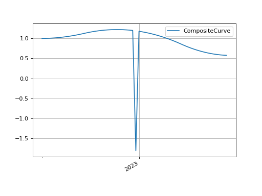
Then we can create a log-cubic curve, with knot points in any valid locations we want and composite this with the turn Curve. Just to be able to display a little more variation instead of a flat curve, a few more rates have been added to create some semblance of shape.

In [13]: log_cubic_curve = Curve(
   ....:     {dt(2022, 12, 1): 1.0, dt(2022, 12, 20): 1.0, dt(2023, 1, 10): 1.0, dt(2023, 1, 31): 1.0},
   ....:     t=[
   ....:        dt(2022, 12, 1), dt(2022, 12, 1), dt(2022, 12, 1), dt(2022, 12, 1),
   ....:        dt(2022, 12, 15),
   ....:        dt(2023, 1, 15),
   ....:        dt(2023, 1, 31), dt(2023, 1, 31), dt(2023, 1, 31), dt(2023, 1, 31)
   ....:     ],
   ....: )
   ....: 

In [14]: composite_curve = CompositeCurve([log_cubic_curve, turn_curve])

In [15]: solver = Solver(
   ....:     curves=[log_cubic_curve, composite_curve],
   ....:     pre_solvers=[turn_solver],
   ....:     instruments=[
   ....:         IRS(dt(2022, 12, 1), "1b", "A", curves=composite_curve),
   ....:         IRS(dt(2022, 12, 20), "1b", "A", curves=composite_curve),
   ....:         IRS(dt(2023, 1, 10), "1b", "A", curves=composite_curve),
   ....:     ],
   ....:     s=[1.0, 1.2, 1.0],
   ....: )
   ....: 
SUCCESS: `func_tol` reached after 2 iterations (levenberg_marquardt), `f_val`: 3.1030712487781767e-15, `time`: 0.0045s

In [16]: composite_curve.plot("1b", labels=["CompositeCurve"])
Out[16]: 
(<Figure size 640x480 with 1 Axes>,
 <Axes: >,
 [<matplotlib.lines.Line2D at 0x7f0a9e6fc6d0>])

(Source code, png, hires.png, pdf)

The Tesla logo is obviously inspired by Swedish design!