Solving Curves with a Dependency Chain#
In real trading environments market-makers and brokers are typically responsible for creating and maintaining their own curves. Normally different teams are responsible for the pricing of different instruments. Some instruments and curves are only dependent upon their local environment, for which a team will have complete visibility. Other instruments might be dependent upon pre-requisite markets to price instruments exactly.
A good example is local currency interest rate curves defined by IRS prices, and cross-currency curves defined by XCS prices but dependent upon FX rates and local currency IRS curves.
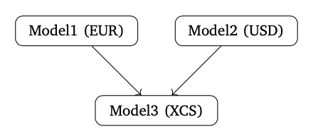
Below, for demonstration purposes we present a minimalist example of a dependency chain constructing EUR and USD interest curves independently and then using them to price a cross-currency model.
The EUR Curve#
The EUR curve is configured and constructed by the EUR IRS team. That team can determine that model in any way they choose.
In the below configuration they have a log linear curve with nodes on 1st May and 1st Jan next year, and these are calibrated exactly with 4M and 1Y swaps whose values are 2% and 2.5%.
In [1]: eureur = Curve(
   ...:     nodes={
   ...:         dt(2022, 1, 1): 1.0,
   ...:         dt(2022, 5, 1): 1.0,
   ...:         dt(2023, 1, 1): 1.0,
   ...:     },
   ...:     convention="act360",
   ...:     calendar="tgt",
   ...:     interpolation="log_linear",
   ...:     id="eureur",
   ...: )
   ...:

In [2]: eur_kws = dict(
   ...:     effective=dt(2022, 1, 3),
   ...:     spec="eur_irs",
   ...:     curves="eureur",
   ...: )
   ...:

In [3]: eur_solver = Solver(
   ...:     curves=[eureur],
   ...:     instruments=[
   ...:         IRS(**eur_kws, termination="4M"),
   ...:         IRS(**eur_kws, termination="1Y"),
   ...:     ],
   ...:     s=[2.0, 2.5],
   ...:     id="eur"
   ...: )
   ...:
SUCCESS: `func_tol` reached after 3 iterations (levenberg_marquardt), `f_val`: 1.1522476203957725e-18, `time`: 0.0021s
The USD Curve#
The same for the USD IRS team. Notice that this model is slightly different for purposes of example. They have a node at the 7M point and also a 7M swap.
In [4]: usdusd = Curve(
   ...:     nodes={
   ...:         dt(2022, 1, 1): 1.0,
   ...:         dt(2022, 8, 1): 1.0,
   ...:         dt(2023, 1, 1): 1.0,
   ...:     },
   ...:     convention="act360",
   ...:     calendar="nyc",
   ...:     interpolation="log_linear",
   ...:     id="usdusd",
   ...: )
   ...:

In [5]: usd_kws = dict(
   ...:     effective=dt(2022, 1, 3),
   ...:     spec="usd_irs",
   ...:     curves="usdusd",
   ...: )
   ...:

In [6]: usd_solver = Solver(
   ...:     curves=[usdusd],
   ...:     instruments=[
   ...:         IRS(**usd_kws, termination="7M"),
   ...:         IRS(**usd_kws, termination="1Y"),
   ...:     ],
   ...:     s=[4.0, 4.8],
   ...:     id="usd"
   ...: )
   ...:
SUCCESS: `func_tol` reached after 3 iterations (levenberg_marquardt), `f_val`: 8.95311645138308e-13, `time`: 0.0024s
The XCS Curve#
The XCS team are then able to rely on these curves, trusting a
construction from their colleagues. The configuration of the XCS curves is
freely chosen by this team. In the configuration the the only linking arguments are
the pre_solver argument and the string id curves references in the instrument
initialisation. An FXForwards object is also created from all
the constructed curves to price forward FX rates for the instruments.
In [7]: fxr = FXRates({"eurusd": 1.10}, settlement=dt(2022, 1, 3))

In [8]: eurusd = Curve(
   ...:     nodes={
   ...:         dt(2022, 1, 1): 1.0,
   ...:         dt(2022, 5, 1): 1.0,
   ...:         dt(2022, 9, 1): 1.0,
   ...:         dt(2023, 1, 1): 1.0,
   ...:     },
   ...:     convention="act360",
   ...:     calendar=None,
   ...:     interpolation="log_linear",
   ...:     id="eurusd",
   ...: )
   ...:

In [9]: fxf = FXForwards(
   ...:     fx_rates=fxr,
   ...:     fx_curves={
   ...:         "usdusd": usdusd,
   ...:         "eureur": eureur,
   ...:         "eurusd": eurusd,
   ...:     }
   ...: )
   ...:

In [10]: xcs_kws = dict(
   ....:     effective=dt(2022, 1, 3),
   ....:     spec="eurusd_xcs",
   ....:     curves=["eureur", "eurusd", "usdusd", "usdusd"]
   ....: )
   ....:

In [11]: xcs_solver = Solver(
   ....:     pre_solvers=[eur_solver, usd_solver],
   ....:     fx=fxf,
   ....:     curves=[eurusd],
   ....:     instruments=[
   ....:         XCS(**xcs_kws, termination="4m"),
   ....:         XCS(**xcs_kws, termination="8m"),
   ....:         XCS(**xcs_kws, termination="1y"),
   ....:     ],
   ....:     s=[-5.0, -6.5, -11.0],
   ....:     id="eur/usd",
   ....: )
   ....:
SUCCESS: `func_tol` reached after 3 iterations (levenberg_marquardt), `f_val`: 1.0572444443750555e-20, `time`: 0.0384s
Back to the EUR Team#
If the EUR team would now need to value and risk an arbitrary swap they are able to do that within their own local model.
In [12]: irs = IRS(**eur_kws, termination="9M", fixed_rate=1.15, notional=100e6)

In [13]: irs.npv(solver=eur_solver)
Out[13]: <Dual: 939767.076623, (eureur0, eureur1, eureur2), [98315131.2, -34950220.0, -64240777.6]>

In [14]: irs.delta(solver=eur_solver)
Out[14]:
local_ccy                    eur
display_ccy                  eur
type        solver label
instruments eur    eur0  1231.09
                   eur1  6115.57
Since their curves are used within the XCS framework this will give precisely the same result if it taken from their model.
In [15]: irs.npv(solver=xcs_solver)
Out[15]: <Dual: 939767.076623, (eureur0, eureur1, eureur2), [98315131.2, -34950220.0, -64240777.6]>

In [16]: irs.delta(solver=xcs_solver)
Out[16]:
local_ccy                        eur
display_ccy                      eur
type        solver  label
instruments eur     eur0     1231.09
                    eur1     6115.57
            usd     usd0        0.00
                    usd1        0.00
            eur/usd eur/usd0    0.00
                    eur/usd1    0.00
                    eur/usd2    0.00
fx          fx      eurusd      0.00
This framework can advance the cause of the EUR team if the swap is collateralised in another currency. For this, the XCS model is definitely required and can be referred to directly:
In [17]: irs.curves = ["eureur", "eurusd"]  # <- changing to a USD CSA for this swap.

In [18]: irs.npv(solver=xcs_solver)
Out[18]: <Dual: 940325.640976, (eureur0, eureur1, eureur2, ...), [98373566.3, -35314844.4, -64892849.8, ...]>

In [19]: irs.delta(solver=xcs_solver)
Out[19]:
local_ccy                        eur
display_ccy                      eur
type        solver  label
instruments eur     eur0     1231.82
                    eur1     6119.22
            usd     usd0       -0.02
                    usd1       -0.03
            eur/usd eur/usd0   -0.35
                    eur/usd1  -48.84
                    eur/usd2  -22.46
fx          fx      eurusd     -0.00
Thus the framework is completely consistent and customisable for all teams to use as required.