Pricing Mechanisms#
This guide is aimed at users who are not completely new to rateslib and who have a little experience already building Instruments, Curves and Solvers are are familiar with some of its basic mechanics already.
Summary#
Rateslib’s API design for valuing and obtaining risk sensitivities of Instruments follows the first two pillars of its design philosophy:
Maximise flexibility : minimise user input,
Prioritise risk sensitivities above valuation.
This means the arguments required for the
Instrument.npv(),
Instrument.delta() and
Instrument.gamma()
are the same and optionally require:
curves, solver, fx, base, local
When calculating risk metrics a solver, which contains derivative mapping information, is
required. However, when calculating value, it is sufficient to just provide curves. In this
case, and if the curves do not contain AD then the calculation might be upto 300% faster.
Since these arguments are optional and can be inferred from each other it is important to understand the combination that can produce results. There are two sections on this page which discuss these combinations.
How
solver,fx,baseandlocalinteract? I.e. what currency will results be displayed in?How
curves,solverand Instruments interact? I.e. which Curves will be used to price which Instruments?
How do solver, fx, base and local interact?#
One of the most important aspects to keep track of when valuing
Instrument.npv() is that
of the currency in which it is displayed. This is the base
currency it is displayed in. base does not need to
be explicitly set to get the results one expects.
The local argument
local can, at any time, be set to True and this will return a dict
containing a currency key and a value. By using this we keep track
of the currency of each Leg of the Instrument. This is important for
risk sensitivities and is used internally, especially for multi-currency instruments.
In [1]: curve = Curve({dt(2022, 1, 1): 1.0, dt(2023, 1, 1): 0.96}, id="curve")

In [2]: fxr = FXRates({"usdeur": 0.9, "gbpusd": 1.25}, base="gbp", settlement=dt(2022, 1, 3))

In [3]: fxf = FXForwards(
   ...:     fx_rates=fxr,
   ...:     fx_curves={"usdusd": curve, "eureur": curve, "gbpgbp": curve, "eurusd": curve, "gbpusd": curve},
   ...:     base="eur",
   ...: )
   ...:

In [4]: solver = Solver(
   ...:     curves=[curve],
   ...:     instruments=[IRS(dt(2022, 1, 1), "1y", "a", curves=curve)],
   ...:     s=[4.109589041095898],
   ...:     fx=fxf,
   ...: )
   ...:
SUCCESS: `func_tol` reached after 0 iterations (levenberg_marquardt), `f_val`: 0.0, `time`: 0.0003s
The below shows the use of the local argument to get the PV of both Legs on this XCS
separately in each currency.
When specifying a base and setting local to False the PV of the Legs are aggregated
and converted to the given currency.
In [5]: nxcs = XCS(dt(2022, 2, 1), "6M", "A", currency="eur", leg2_currency="usd", leg2_mtm=False)

In [6]: nxcs.npv(curves=[curve]*4, fx=fxf, local=True)
Out[6]:
{'usd': <Dual: -4.962793, (fx_gbpusd, fx_usdeur, curve1, ...), [0.0, 5.5, 251.5, ...]>,
 'eur': <Dual: 4.466513, (curve1, curve0), [-226.4, 221.8]>}

In [7]: nxcs.npv(curves=[curve]*4, fx=fxf, base="usd")
Out[7]: <Dual: 0.000000, (fx_gbpusd, fx_usdeur, curve1, ...), [0.0, 0.0, 0.0, ...]>
What is best practice?#
For single currency Instruments, if you want to return an npv value in its local currency
then you do not need to supply base or fx arguments. However, to
be explicit, base can also be specified.
In [8]: irs = IRS(dt(2022, 2, 1), "6M", "A", currency="usd", fixed_rate=4.0, curves=curve)

In [9]: irs.npv(solver=solver)              # USD is local currency default, solver.fx.base is EUR.
Out[9]: <Dual: 330.405115, (curve1, curve0), [-514447.8, 494200.3]>

In [10]: irs.npv(solver=solver, base="usd")  # USD is explicit, solver.fx.base is EUR.
Out[10]: <Dual: 330.405115, (curve1, curve0), [-514447.8, 494200.3]>
To calculate a value in another non-local currency supply an fx object and
specify the base. It is not good practice to supply fx as numeric since this
can result in errors (if the exchange rate is given the wrong way round (human error))
and it does not preserve AD or any FX sensitivities. base is inferred from the
fx object so the following are all equivalent. fx objects are commonly inherited from
solvers.
In [11]: irs.npv(fx=fxr)                     # GBP is fx's base currency
Out[11]: <Dual: 264.324092, (curve1, curve0, fx_gbpusd, ...), [-411558.2, 395360.2, -211.5, ...]>

In [12]: irs.npv(fx=fxr, base="gbp")         # GBP is explicitly specified
Out[12]: <Dual: 264.324092, (curve1, curve0, fx_gbpusd, ...), [-411558.2, 395360.2, -211.5, ...]>

In [13]: irs.npv(fx=fxr, base=fxr.base)      # GBP is fx's base currency
Out[13]: <Dual: 264.324092, (curve1, curve0, fx_gbpusd, ...), [-411558.2, 395360.2, -211.5, ...]>

In [14]: irs.npv(solver=solver, base="gbp")  # GBP is explicitly specified
Out[14]: <Dual: 264.324092, (fx_gbpusd, fx_usdeur, curve1, ...), [-211.5, 0.0, -411558.2, ...]>
For multi-currency Instruments, which include FXSwaps, FXExchanges and XCSs, these
instruments typically rely on an FXForwards object to value correctly, in which case that will be
supplied either via solver or via the fx argument. base can be set explicitly,
or set as the same as fx.base, or it will be taken as the local Leg1 currency.
Technical rules#
If base is not given it will be inferred from one of two objects;
either it will be inferred from the provided
fxobject,or it will be inferred from the Leg or from Leg1 of an Instrument.
base will not be inherited from a second layer inherited object. I.e. base
will not be set equal to the base currency of the solver.fx associated object.
Case and Output |
|
|
|
|
|---|---|---|---|---|
|
||||
Returns if currency and |
X |
X |
||
Returns and warns about best practice. |
X |
(numeric) |
||
Returns if currency and |
X |
X |
||
Returns if currency and |
X |
X |
X |
|
Returns if |
X |
|||
Returns if |
X |
X |
||
|
||||
Returns inferring |
<- |
X |
||
Returns inferring |
<- |
X |
X |
|
Returns inferring |
<- |
X |
X |
|
Returns inferring |
(local) |
X |
||
Returns inferring |
(local) |
X |
||
Returns inferring |
(local) |
Examples#
We continue the examples above using the USD IRS created and consider possible npvs:
In [15]: def npv(irs, curves=NoInput(0), solver=NoInput(0), fx=NoInput(0), base=NoInput(0)):
   ....:    try:
   ....:       _ = irs.npv(curves, solver, fx, base)
   ....:    except Exception as e:
   ....:       _ = str(e)
   ....:    return _
   ....:
# The following are all explicit EUR output
In [16]: npv(irs, base="eur")          # Error since no conversion rate available.
Out[16]: "`base` (eur) cannot be requested without supplying `fx` as a valid FXRates or FXForwards object to convert to currency (usd).\nIf you are using a `Solver` with multi-currency instruments have you forgotten to attach the FXForwards in the solver's `fx` argument?"

In [17]: npv(irs, base="eur", fx=fxr)  # Takes 0.9 FX rate from object.
Out[17]: <Dual: 297.364604, (curve1, curve0, fx_gbpusd, ...), [-463003.0, 444780.2, 0.0, ...]>

In [18]: npv(irs, base="eur", fx=2.0)  # UserWarning and no fx Dual sensitivities.
Out[18]: <Dual: 660.810231, (curve1, curve0), [-1028895.5, 988400.5]>

In [19]: npv(irs, base="eur", solver=solver)  # Takes 0.95 FX rates from solver.fx
Out[19]: <Dual: 297.364604, (fx_gbpusd, fx_usdeur, curve1, ...), [0.0, 330.4, -463003.0, ...]>

In [20]: npv(irs, base="eur", fx=fxr, solver=solver)  # Takes 0.9 FX rate from fx
Out[20]: <Dual: 297.364604, (curve1, curve0, fx_gbpusd, ...), [-463003.0, 444780.2, 0.0, ...]>

# The following infer the base
In [21]: npv(irs)                         # Base is inferred as local currency: USD
Out[21]: <Dual: 330.405115, (curve1, curve0), [-514447.8, 494200.3]>

In [22]: npv(irs, fx=fxr)                 # Base is inferred from fx: GBP
Out[22]: <Dual: 264.324092, (curve1, curve0, fx_gbpusd, ...), [-411558.2, 395360.2, -211.5, ...]>

In [23]: npv(irs, fx=fxr, base=fxr.base)  # Base is explicit from fx: GBP
Out[23]: <Dual: 264.324092, (curve1, curve0, fx_gbpusd, ...), [-411558.2, 395360.2, -211.5, ...]>

In [24]: npv(irs, fx=fxr, solver=solver)  # Base is inferred from fx: GBP. UserWarning for different fx objects
Out[24]: <Dual: 264.324092, (curve1, curve0, fx_gbpusd, ...), [-411558.2, 395360.2, -211.5, ...]>

In [25]: npv(irs, solver=solver)          # Base is inferred as local currency: USD
Out[25]: <Dual: 330.405115, (curve1, curve0), [-514447.8, 494200.3]>

In [26]: npv(irs, solver=solver, fx=solver.fx)  # Base is inferred from solver.fx: EUR
Out[26]: <Dual: 264.324092, (fx_gbpusd, fx_usdeur, curve1, ...), [-211.5, 0.0, -411558.2, ...]>
How curves, solver and Instruments interact?#
The pricing mechanisms in rateslib require Instruments and
Curves. FX objects
(usually FXForwards) may also be required
(for multi-currency instruments), and these
are all often interdependent and calibrated by a Solver.
Since Instruments are separate objects to Curves and Solvers, when pricing them it requires a mapping to link them all together. This leads to…
Three different modes of initialising an Instrument:
Dynamic - Price Time Mapping: this means an Instrument is initialised without any
curvesand these must be provided later at price time, usually inside a function call.In [27]: instrument = IRS(dt(2022, 1, 1), "10Y", "A", fixed_rate=2.5) In [28]: curve = Curve({dt(2022, 1, 1): 1.0, dt(2032, 1, 1): 0.85}) In [29]: instrument.npv(curves=curve) Out[29]: -82171.04166115227 In [30]: instrument.rate(curves=curve) Out[30]: 1.6151376354769178
Explicit - Immediate Mapping: this means an Instrument is initialised with
curvesand this object will be used if no Curves are provided at price time. The Curves must already exist when initialising the Instrument.In [31]: curve = Curve({dt(2022, 1, 1): 1.0, dt(2032, 1, 1): 0.85}) In [32]: instrument = IRS(dt(2022, 1, 1), "10Y", "A", fixed_rate=2.5, curves=curve) In [33]: instrument.npv() Out[33]: -82171.04166115227 In [34]: instrument.rate() Out[34]: 1.6151376354769178
Indirect - String
idMapping: this means an Instrument is initialised withcurvesthat contain lookup information to collect the Curves at price time from asolver.In [35]: instrument = IRS(dt(2022, 1, 1), "10Y", "A", fixed_rate=2.5, curves="curve-id") In [36]: curve = Curve({dt(2022, 1, 1): 1.0, dt(2032, 1, 1): 0.85}, id="curve-id") In [37]: solver = Solver( ....: curves=[curve], ....: instruments=[IRS(dt(2022, 1, 1), "10Y", "A", curves=curve)], ....: s=[1.6151376354769178] ....: ) ....: SUCCESS: `func_tol` reached after 0 iterations (levenberg_marquardt), `f_val`: 1.779867417404908e-29, `time`: 0.0015s In [38]: instrument.npv(solver=solver) Out[38]: <Dual: -82171.041661, (curve-id1, curve-id0), [-1146523.3, 892373.8]> In [39]: instrument.rate(solver=solver) Out[39]: <Dual: 1.615138, (curve-id1, curve-id0), [-11.8, 10.0]>
Then, for price time, this then also leads to the following cases…
Two modes of pricing an Instrument:
Direct Curves Override: if
curvesare given dynamically these are used regardless of which initialisation mode was used for the Instrument.In [40]: curve = Curve({dt(2022, 1, 1): 1.0, dt(2032, 1, 1): 0.85}) In [41]: irs = IRS(dt(2022, 1, 1), "10Y", "A", curves=curve) In [42]: other_curve = Curve({dt(2022, 1, 1): 1.0, dt(2032, 1, 1): 0.85}) In [43]: irs.npv(curves=other_curve) # other_curve overrides the initialised curve Out[43]: -2.9103830456733704e-11 In [44]: irs.rate(curves=other_curve) # other_curve overrides the initialised curve Out[44]: 1.6151376354769178
With Default Initialisation: if
curvesat price time are not provided then those specified at initialisation are used.As Objects: if Curves were specified these are used directly (see 2. above)
From String id with Solver: if
curvesare not objects, but strings, then asolvermust be supplied to extract the Curves from (see 3. above).
In the unusual combination that curves are given directly in combination with a solver,
and those curves do not form part of the solver’s curve collection, then depending upon the
rateslib options configured, then errors or warnings might be raised or this might be ignored.
What is best practice?#
Amongst the variety of input pricing methods there is a recommended way of working.
This is to use method 3) and to initialise Instruments with a defined curves argument
as string id s. This does not
impede dynamic pricing if curves are constructed and supplied later directly to
pricing methods.
The curves attribute on the Instrument is instructive of its pricing intent.
In [45]: irs = IRS(
   ....:     effective=dt(2022, 1, 1),
   ....:     termination="6m",
   ....:     frequency="Q",
   ....:     currency="usd",
   ....:     notional=500e6,
   ....:     fixed_rate=2.0,
   ....:     curves="sofr",  # or ["sofr", "sofr"] for forecasting and discounting
   ....: )
   ....:

In [46]: irs.curves
Out[46]: 'sofr'
At any point a Curve could be constructed and used for dynamic pricing, even if
its id does not match the instrument initialisation. This is usually used in sampling or
scenario analysis.
In [47]: curve = Curve(
   ....:     nodes={dt(2022, 1, 1): 1.0, dt(2023, 1, 1): 0.98},
   ....:     id="not_sofr"
   ....: )
   ....:

In [48]: irs.rate(curve)
Out[48]: 1.9975948370062162
Why is this best practice?#
The reasons that this is best practice are:
It provides more flexibility when working with multiple different curve models and multiple
Solvers. Instruments do not need to be re-initialised just to extract alternate valuations or alternate risk sensitivities.It provides more flexibility since only Instruments constructed in this manner can be directly added to the
Portfolioclass. It also extends theSpreadandFlyclasses to allow Instruments which do not share the same Curves.It removes the need to externally keep track of the necessary pricing curves needed for each instrument created, which is often four curves for two legs.
It creates redundancy by avoiding programmatic errors when curves are overwritten and object oriented associations are silently broken, which can occur when using the other methods.
It is anticipated that this mechanism is the one most future proofed when rateslib is extended for server-client-api transfer via JSON or otherwise.
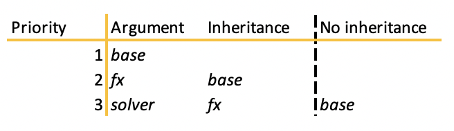
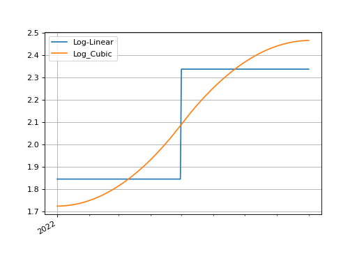
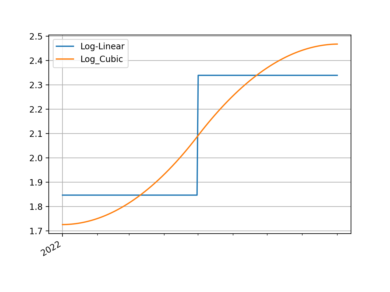
Multiple curve model Solvers#
Consider two different curve models, a log-linear one and a log-cubic spline, which we calibrate with the same instruments.
In [49]: instruments = [
   ....:     IRS(dt(2022, 1, 1), "4m", "Q", curves="sofr"),
   ....:     IRS(dt(2022, 1, 1), "8m", "Q", curves="sofr"),
   ....: ]
   ....:

In [50]: s = [1.85, 2.10]

In [51]: ll_curve = Curve(
   ....:     nodes={
   ....:         dt(2022, 1, 1): 1.0,
   ....:         dt(2022, 5, 1): 1.0,
   ....:         dt(2022, 9, 3): 1.0
   ....:     },
   ....:     interpolation="log_linear",
   ....:     id="sofr"
   ....: )
   ....:

In [52]: lc_curve = Curve(
   ....:     nodes={
   ....:         dt(2022, 1, 1): 1.0,
   ....:         dt(2022, 5, 1): 1.0,
   ....:         dt(2022, 9, 3): 1.0
   ....:     },
   ....:     t=[dt(2022, 1, 1), dt(2022, 1, 1), dt(2022, 1, 1), dt(2022, 1, 1),
   ....:        dt(2022, 5, 1),
   ....:        dt(2022, 9, 3), dt(2022, 9, 3), dt(2022, 9, 3), dt(2022, 9, 3)],
   ....:     id="sofr",
   ....: )
   ....:

In [53]: ll_solver = Solver(curves=[ll_curve], instruments=instruments, s=s, instrument_labels=["4m", "8m"], id="sofr")
SUCCESS: `func_tol` reached after 3 iterations (levenberg_marquardt), `f_val`: 1.0687768947368452e-16, `time`: 0.0041s

In [54]: lc_solver = Solver(curves=[lc_curve], instruments=instruments, s=s, instrument_labels=["4m", "8m"], id="sofr")
SUCCESS: `func_tol` reached after 3 iterations (levenberg_marquardt), `f_val`: 1.2711948339281648e-16, `time`: 0.0038s

In [55]: ll_curve.plot("1D", comparators=[lc_curve], labels=["LL Curve", "LC Curve"])
Out[55]:
(<Figure size 640x480 with 1 Axes>,
 <Axes: >,
 [<matplotlib.lines.Line2D at 0x7f0a9f1c6210>,
  <matplotlib.lines.Line2D at 0x7f0a9ef28410>])
(Source code, png, hires.png, pdf)

Since the irs instrument was initialised indirectly with string id s we can
supply the Solver s as pricing parameters and the curves named “sofr” in each
of them will be looked up and used to price the irs.
In [56]: irs.rate(solver=ll_solver)
Out[56]: <Dual: 2.017016, (sofr0, sofr1, sofr2), [200.1, -103.5, -98.7]>

In [57]: irs.rate(solver=lc_solver)
Out[57]: <Dual: 1.984736, (sofr0, sofr1, sofr2), [220.2, -143.1, -79.1]>
The Dual datatypes already hint at different risk sensitivities
of the instrument under the different curve model solvers. For good order we can
display the delta risks.
In [58]: irs.delta(solver=ll_solver)
Out[58]:
local_ccy                     usd
display_ccy                   usd
type        solver label
instruments sofr   4m     8341.36
                   8m    16622.06

In [59]: irs.delta(solver=lc_solver)
Out[59]:
local_ccy                     usd
display_ccy                   usd
type        solver label
instruments sofr   4m    11573.70
                   8m    13397.65
The programmatic errors avoided are as follows:
In [60]: try:
   ....:     irs.delta(curves=ll_curve, solver=lc_solver)
   ....: except Exception as e:
   ....:     print(e)
   ....:
A curve has been supplied, as part of ``curves``, which has the same `id` ('sofr'),
as one of the curves available as part of the Solver's collection but is not the same object.
This is ambiguous and cannot price.
Either refactor the arguments as follows:
1) remove the conflicting curve: [curves=[..], solver=<Solver>] -> [curves=None, solver=<Solver>]
2) change the `id` of the supplied curve and ensure the rateslib.defaults option 'curve_not_in_solver' is set to 'ignore'.
   This will remove the ability to accurately price risk metrics.
Using a Portfolio#
We can consider creating another Solver for the ESTR curve which extends the SOFR
solver.
In [61]: instruments = [
   ....:     IRS(dt(2022, 1, 1), "3m", "Q", curves="estr"),
   ....:     IRS(dt(2022, 1, 1), "9m", "Q", curves="estr"),
   ....: ]
   ....:

In [62]: s = [0.75, 1.65]

In [63]: ll_curve = Curve(
   ....:     nodes={
   ....:         dt(2022, 1, 1): 1.0,
   ....:         dt(2022, 4, 1): 1.0,
   ....:         dt(2022, 10, 1): 1.0
   ....:     },
   ....:     interpolation="log_linear",
   ....:     id="estr",
   ....: )
   ....:

In [64]: combined_solver = Solver(
   ....:     curves=[ll_curve],
   ....:     instruments=instruments,
   ....:     s=s,
   ....:     instrument_labels=["3m", "9m"],
   ....:     pre_solvers=[ll_solver],
   ....:     id="estr"
   ....: )
   ....:
SUCCESS: `func_tol` reached after 3 iterations (levenberg_marquardt), `f_val`: 1.237437454456797e-15, `time`: 0.0032s
Now we create another IRS and add it to a
Portfolio
In [65]: irs2 = IRS(
   ....:     effective=dt(2022, 1, 1),
   ....:     termination="6m",
   ....:     frequency="Q",
   ....:     currency="eur",
   ....:     notional=-300e6,
   ....:     fixed_rate=1.0,
   ....:     curves="estr",
   ....: )
   ....:

In [66]: pf = Portfolio([irs, irs2])

In [67]: pf.npv(solver=combined_solver, local=True)
Out[67]:
{'usd': <Dual: 42456.377860, (sofr0, sofr1, sofr2), [499326346.8, -258138138.0, -246219539.0]>,
 'eur': <Dual: -638082.239972, (estr0, estr1, estr2), [-299965158.7, 151143418.5, 150334069.1]>}

In [68]: pf.delta(solver=combined_solver)
Out[68]:
local_ccy                      eur      usd
display_ccy                    eur      usd
type        solver label
instruments sofr   4m         0.00  8341.36
                   8m         0.00 16622.06
            estr   3m     -3741.35     0.00
                   9m    -11247.59     0.00

In [69]: pf.gamma(solver=combined_solver)
Out[69]:
type                                           instruments
solver                                                sofr       estr
label                                                   4m    8m   3m   9m
local_ccy display_ccy type        solver label
eur       eur         instruments sofr   4m           0.00  0.00 0.00 0.00
                                         8m           0.00  0.00 0.00 0.00
                                  estr   3m           0.00  0.00 0.14 0.28
                                         9m           0.00  0.00 0.28 0.44
usd       usd         instruments sofr   4m          -0.32 -0.50 0.00 0.00
                                         8m          -0.50 -0.52 0.00 0.00
                                  estr   3m           0.00  0.00 0.00 0.00
                                         9m           0.00  0.00 0.00 0.00
Warnings#
Silently breaking object associations#
Warning
There is no redundancy for breaking object oriented associations when an
Instrument is initialised with curves as objects.
When an Instrument is created with a direct object
association to Curves which have already been constructed. These will then be
used by default when pricing.
In [70]: curve = Curve({dt(2022, 1, 1): 1.0, dt(2023, 1, 1): 0.98})

In [71]: irs = IRS(dt(2022, 1, 1), "6m", "Q", currency="usd", fixed_rate=2.0, curves=curve)

In [72]: irs.rate()
Out[72]: 1.9975948370062162

In [73]: irs.npv()
Out[73]: -12.0008132132225
If the object is overwritten, or is recreated (say, as a new Curve) the results
will not be as expected.
In [74]: curve = "bad_object"  # overwrite the curve variable but the object still exists.

In [75]: irs.rate()
Out[75]: 1.9975948370062162
It is required to update objects instead of recreating them. The documentation
for FXForwards.update() also elaborates
on this point.
Disassociated objects#
Warning
Combining curves and solver that are not associated is bad practice. There
are options for trying to avoid this behaviour.
Consider the below example, which includes two Curve s
and a Solver.
One Curve, labelled “ibor”, is independent, the other,
labelled “rfr”, is associated with the Solver, since it has
been iteratively solved.
In [76]: rfr_curve = Curve({dt(2022, 1, 1): 1.0, dt(2023, 1, 1): 0.98}, id="rfr")

In [77]: ibor_curve = Curve({dt(2022, 1, 1): 1.0, dt(2023, 1, 1): 0.97}, id="ibor")

In [78]: solver = Solver(
   ....:     curves=[rfr_curve],
   ....:     instruments=[(Value(dt(2023, 1, 1)), ("rfr",), {})],
   ....:     s=[0.9825]
   ....: )
   ....:
SUCCESS: `func_tol` reached after 8 iterations (levenberg_marquardt), `f_val`: 2.3630340650323354e-14, `time`: 0.0012s
When the option curve_not_in_solver is set to “ignore” the independent
Curve and a disassociated Solver
can be provided to a pricing method and the output returns. It uses the curve and,
effectively, ignores the disassociated solver.
In [79]: irs = IRS(dt(2022, 1, 1), dt(2023, 1, 1), "A")

In [80]: defaults.curve_not_in_solver = "ignore"

In [81]: irs.rate(ibor_curve, solver)
Out[81]: 3.050416607823765
In the above the solver is not used for pricing, since it is decoupled from
ibor_curve. It is technically an error to list it as an argument.
Setting the option to “warn” or “raise” enforces a UserWarning or a
ValueError when this behaviour is detected.
In [82]: defaults.curve_not_in_solver = "raise"

In [83]: try:
   ....:     irs.rate(ibor_curve, solver)
   ....: except Exception as e:
   ....:     print(e)
   ....:
`curve` must be in `solver`.
When referencing objects by id s this becomes immediately apparent since, the
below will always fail regardless of the configurable option (the solver does not
contain the requested curve and therefore cannot fulfill the request).
In [84]: defaults.curve_not_in_solver = "ignore"

In [85]: try:
   ....:     irs.rate("ibor", solver)
   ....: except Exception as e:
   ....:     print(e)
   ....:
`curves` must contain str curve `id` s existing in `solver` (or its associated `pre_solvers`)