CompositeCurve#

class rateslib.curves.CompositeCurve(curves, id=NoInput.blank)#

Bases: IndexCurve

A dynamic composition of a sequence of other curves.

Note

Can only composite curves of the same type: Curve, IndexCurve or LineCurve. Other curve parameters such as modifier, calendar and convention must also match.

Parameters:

curves (sequence of Curve, LineCurve or IndexCurve) – The curves to be composited.
id (str, optional, set by Default) – The unique identifier to distinguish between curves in a multi-curve framework.

Examples

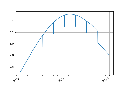
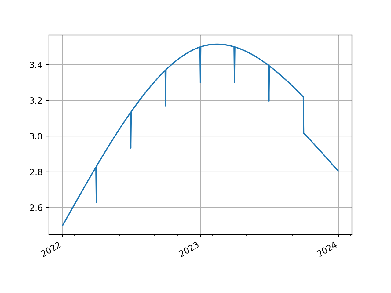
Composite two LineCurve s. Here, simulating the effect of adding quarter-end turns to a cubic spline interpolator, which is otherwise difficult to mathematically derive.

In [1]: from rateslib.curves import LineCurve, CompositeCurve

In [2]: line_curve1 = LineCurve(
   ...:     nodes={
   ...:         dt(2022, 1, 1): 2.5,
   ...:         dt(2023, 1, 1): 3.5,
   ...:         dt(2024, 1, 1): 3.0,
   ...:     },
   ...:     t=[dt(2022, 1, 1), dt(2022, 1, 1), dt(2022, 1, 1), dt(2022, 1, 1),
   ...:        dt(2023, 1, 1),
   ...:        dt(2024, 1, 1), dt(2024, 1, 1), dt(2024, 1, 1), dt(2024, 1, 1)],
   ...: )
   ...: 

In [3]: line_curve2 = LineCurve(
   ...:     nodes={
   ...:         dt(2022, 1, 1): 0,
   ...:         dt(2022, 3, 31): -0.2,
   ...:         dt(2022, 4, 1): 0,
   ...:         dt(2022, 6, 30): -0.2,
   ...:         dt(2022, 7, 1): 0,
   ...:         dt(2022, 9, 30): -0.2,
   ...:         dt(2022, 10, 1): 0,
   ...:         dt(2022, 12, 31): -0.2,
   ...:         dt(2023, 1, 1): 0,
   ...:         dt(2023, 3, 31): -0.2,
   ...:         dt(2023, 4, 1): 0,
   ...:         dt(2023, 6, 30): -0.2,
   ...:         dt(2023, 7, 1): 0,
   ...:         dt(2023, 9, 30): -0.2,
   ...:     },
   ...:     interpolation="flat_forward",
   ...: )
   ...: 

In [4]: curve = CompositeCurve([line_curve1, line_curve2])

In [5]: curve.plot("1d")
Out[5]: 
(<Figure size 640x480 with 1 Axes>,
 <Axes: >,
 [<matplotlib.lines.Line2D at 0x7f0aac4498d0>])

(Source code, png, hires.png, pdf)

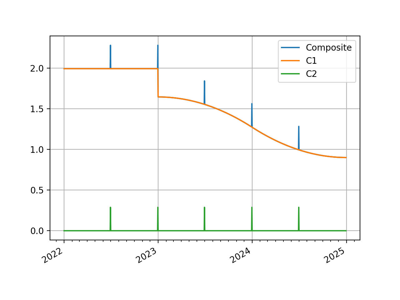
../_images/rateslib-curves-CompositeCurve-1.png

We can also composite DF based curves by using a fast approximation or an exact match.

In [6]: from rateslib.curves import Curve, CompositeCurve

In [7]: curve1 = Curve(
   ...:     nodes={
   ...:         dt(2022, 1, 1): 1.0,
   ...:         dt(2023, 1, 1): 0.98,
   ...:         dt(2024, 1, 1): 0.965,
   ...:         dt(2025, 1, 1): 0.955
   ...:     },
   ...:     t=[dt(2023, 1, 1), dt(2023, 1, 1), dt(2023, 1, 1), dt(2023, 1, 1),
   ...:        dt(2024, 1, 1),
   ...:        dt(2025, 1, 1), dt(2025, 1, 1), dt(2025, 1, 1), dt(2025, 1, 1)],
   ...: )
   ...: 

In [8]: curve2 =Curve(
   ...:     nodes={
   ...:         dt(2022, 1, 1): 1.0,
   ...:         dt(2022, 6, 30): 1.0,
   ...:         dt(2022, 7, 1): 0.999992,
   ...:         dt(2022, 12, 31): 0.999992,
   ...:         dt(2023, 1, 1): 0.999984,
   ...:         dt(2023, 6, 30): 0.999984,
   ...:         dt(2023, 7, 1): 0.999976,
   ...:         dt(2023, 12, 31): 0.999976,
   ...:         dt(2024, 1, 1): 0.999968,
   ...:         dt(2024, 6, 30): 0.999968,
   ...:         dt(2024, 7, 1): 0.999960,
   ...:         dt(2025, 1, 1): 0.999960,
   ...:     },
   ...: )
   ...: 

In [9]: curve = CompositeCurve([curve1, curve2])

In [10]: curve.plot("1D", comparators=[curve1, curve2], labels=["Composite", "C1", "C2"])
Out[10]: 
(<Figure size 640x480 with 1 Axes>,
 <Axes: >,
 [<matplotlib.lines.Line2D at 0x7f0aa5524e90>,
  <matplotlib.lines.Line2D at 0x7f0aa5533b10>,
  <matplotlib.lines.Line2D at 0x7f0aa5540490>])

(Source code, png, hires.png, pdf)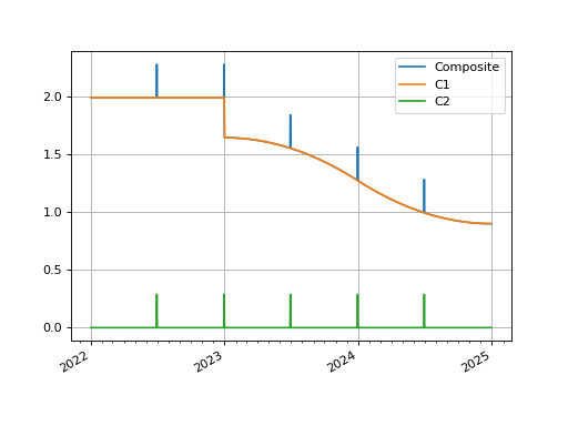

../_images/rateslib-curves-CompositeCurve-2.png

The rate() method of a CompositeCurve composed of either Curve or IndexCurve s accepts an approximate argument. When True by default it used a geometric mean approximation to determine composite period rates. Below we demonstrate this is more than 1000x faster and within 1e-8 of the true value.

In [11]: curve.rate(dt(2022, 6, 1), "1y")
Out[11]: 1.859031948251767

In [12]: %timeit curve.rate(dt(2022, 6, 1), "1y")
72.8 us +- 797 ns per loop (mean +- std. dev. of 7 runs, 10,000 loops each)

In [13]: curve.rate(dt(2022, 6, 1), "1y", approximate=False)
Out[13]: 1.85903194144122

In [14]: %timeit curve.rate(dt(2022, 6, 1), "1y", approximate=False)
45.4 ms +- 1.51 ms per loop (mean +- std. dev. of 7 runs, 10 loops each)

Attributes Summary

collateral

Methods Summary

`copy`()	Create an identical copy of the curve object.
`csolve`()	Solves and sets the coefficients, `c`, of the `PPSpline`.
`from_json`(curve, **kwargs)	Reconstitute a curve from JSON.
`index_value`(date[, interpolation])	Calculate the accrued value of the index from the `index_base`.
`plot`(tenor[, right, left, comparators, ...])	Plot given forward tenor rates from the curve.
`plot_index`([right, left, comparators, ...])	Plot given forward tenor rates from the curve.
`rate`(effective[, termination, modifier, ...])	Calculate the composited rate on the curve.
`roll`(tenor)	Create a new curve with its shape translated in time
`shift`(spread[, id, composite, collateral])	Create a new curve by vertically adjusting the curve by a set number of basis points.
`to_json`()	Convert the parameters of the curve to JSON format.
`translate`(start[, t])	Create a new curve with an initial node date moved forward keeping all else constant.

Attributes Documentation

collateral = None#

Methods Documentation

copy()#

Create an identical copy of the curve object.

Return type:: Curve or LineCurve

csolve()#

Solves and sets the coefficients, c, of the PPSpline.

Return type:: None

Notes

Only impacts curves which have a knot sequence, t, and a PPSpline. Only solves if c not given at curve initialisation.

Uses the spline_endpoints attribute on the class to determine the solving method.

classmethod from_json(curve, **kwargs)#

Reconstitute a curve from JSON.

Parameters:: curve (str) – The JSON string representation of the curve.
Return type:: Curve or LineCurve

index_value(date, interpolation='daily')#

Calculate the accrued value of the index from the index_base.

See IndexCurve.index_value()

plot(tenor, right=NoInput.blank, left=NoInput.blank, comparators=[], difference=False, labels=[])#

Plot given forward tenor rates from the curve.

Parameters:

tenor (str) – The tenor of the forward rates to plot, e.g. “1D”, “3M”.
right (datetime or str, optional) – The right bound of the graph. If given as str should be a tenor format defining a point measured from the initial node date of the curve. Defaults to the final node of the curve minus the tenor.
left (datetime or str, optional) – The left bound of the graph. If given as str should be a tenor format defining a point measured from the initial node date of the curve. Defaults to the initial node of the curve.
comparators (list[Curve]) – A list of curves which to include on the same plot as comparators.
difference (bool) – Whether to plot as comparator minus base curve or outright curve levels in plot. Default is False.
labels (list[str]) – A list of strings associated with the plot and comparators. Must be same length as number of plots.

Returns:

(fig, ax, line)

Return type:

Matplotlib.Figure, Matplotplib.Axes, Matplotlib.Lines2D

plot_index(right=NoInput.blank, left=NoInput.blank, comparators=[], difference=False, labels=[])#

Plot given forward tenor rates from the curve.

Parameters:

tenor (str) – The tenor of the forward rates to plot, e.g. “1D”, “3M”.
right (datetime or str, optional) – The right bound of the graph. If given as str should be a tenor format defining a point measured from the initial node date of the curve. Defaults to the final node of the curve minus the tenor.
left (datetime or str, optional) – The left bound of the graph. If given as str should be a tenor format defining a point measured from the initial node date of the curve. Defaults to the initial node of the curve.
comparators (list[Curve]) – A list of curves which to include on the same plot as comparators.
difference (bool) – Whether to plot as comparator minus base curve or outright curve levels in plot. Default is False.
labels (list[str]) – A list of strings associated with the plot and comparators. Must be same length as number of plots.

Returns:

(fig, ax, line)

Return type:

Matplotlib.Figure, Matplotplib.Axes, Matplotlib.Lines2D

rate(effective, termination=None, modifier=False, approximate=True)#

Calculate the composited rate on the curve.

If rates are sought for dates prior to the initial node of the curve None will be returned.

Parameters:

effective (datetime) – The start date of the period for which to calculate the rate.
termination (datetime or str) – The end date of the period for which to calculate the rate.
modifier (str, optional) – The day rule if determining the termination from tenor. If False is determined from the Curve modifier.
approximate (bool, optional) – When compositing Curve or IndexCurve calculating many individual rates is expensive. This uses an approximation typically with error less than 1/100th of basis point. Not used if multi_csa is True.

Return type:

Dual, Dual2 or float

roll(tenor)#

Create a new curve with its shape translated in time

This curve adjustment is a simulation of a future state of the market where forward rates are assumed to have moved so that the present day’s curve shape is reflected in the future (or the past). This is often used in trade strategy analysis.

Parameters:: tenor (datetime or str) – The date or tenor by which to roll the curve. If a tenor, as str, will derive the datetime as measured from the initial node date. If supplying a negative tenor, or a past datetime, there is a limit to how far back the curve can be rolled - it will first roll backwards and then attempt to translate() forward to maintain the initial node date.
Return type:: CompositeCurve

shift(spread, id=None, composite=True, collateral=None)#

Create a new curve by vertically adjusting the curve by a set number of basis points.

This curve adjustment preserves the shape of the curve but moves it up or down as a translation. This method is suitable as a way to assess value changes of instruments when a parallel move higher or lower in yields is predicted.

Parameters:

spread (float, Dual, Dual2) – The number of basis points added to the existing curve.
id (str, optional) – Set the id of the returned curve.
composite (bool, optional) – If True will return a CompositeCurve that adds a flat curve to the existing curve. This results in slower calculations but the curve will maintain a dynamic association with the underlying curve and will change if the underlying curve changes.
collateral (str, optional) – Designate a collateral tag for the curve which is used by other methods.

Return type:

CompositeCurve

to_json()#

Convert the parameters of the curve to JSON format.

Return type:: str

translate(start, t=False)#

Create a new curve with an initial node date moved forward keeping all else constant.

This curve adjustment preserves forward curve expectations as time evolves. This method is suitable as a way to create a subsequent opening curve from a previous day’s closing curve.

Parameters:

start (datetime) – The new initial node date for the curve, must be in the domain: (node_date[0], node_date[1]]
t (bool) – Set to True if the initial knots of the knot sequence should be translated forward.

Return type:

CompositeCurve