Piecewise Polynomial Splines#

Th rateslib.splines module implements the library’s own piecewise polynomial splines of generic order such that we can include it within our Curve class for log-cubic discount factor interpolation. It does this using b-splines, and various named splines are compatible with Dual and Dual2 data types for automatic differentiation.

The calculations are based on the material provided in A Practical Guide to Splines by Carl de Boor.

`rateslib.splines.PPSplineF64`(k, t[, c])	Piecewise polynomial spline composed of float values on the x and y axes.
`rateslib.splines.PPSplineDual`(k, t[, c])	Piecewise polynomial spline composed of float values on the x-axis and Dual values on the y-axis.
`rateslib.splines.PPSplineDual2`(k, t[, c])	Piecewise polynomial spline composed of float values on the x-axis and Dual2 values on the y-axis.

For legacy reasons PPSpline is now an alias for PPSplineF64 which allows only float-64 (x,y) values.

Introduction#

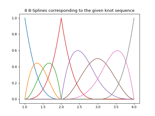
A spline function is one which is composed of a sum of other polynomial functions. In this case, the spline function, $\$(x)$, is a linear sum of b-splines.

\[\$(x) = \sum_{i=1}^n c_i B_{i, k, \mathbf{t}}(x)\]

Below we plot the 8 b-splines associated with the example knot sequence,

t: [1,1,1,1,2,2,2,3,4,4,4,4] (the knot sequence)
k: 4 (the order of the spline (cubic))
$\mathbf{\xi}$ : {1, 2, 3, 4} (the breakpoints sequence)
$\mathbf{\nu}$: {1, 3} (the number of interior continuity conditions)
n: 8 (the dimension of the spline, also degrees of freedom)

In [1]: t = [1,1,1,1,2,2,2,3,4,4,4,4]

In [2]: spline = PPSplineF64(k=4, t=t)

In [3]: x = np.linspace(1, 4, 76)

In [4]: fig, ax = plt.subplots(1,1)

In [5]: for i in range(spline.n):
   ...:     ax.plot(x, spline.bsplev(x, i))
   ...: 

(Source code, png, hires.png, pdf)

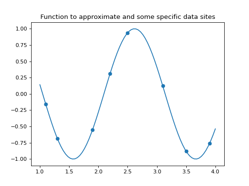
Suppose we now have a function, $g(x)$, within the domain [1,4], eg $g(x)=sin(3x)$ and we sample 8 data sites, $\mathbf{\tau}$, within the domain for the function value:

In [6]: tau = np.array([1.1, 1.3, 1.9, 2.2, 2.5, 3.1, 3.5, 3.9])

In [7]: fig, ax = plt.subplots(1,1)

In [8]: ax.plot(x, np.sin(3*x))
Out[8]: [<matplotlib.lines.Line2D at 0x7f0aa01f01d0>]

In [9]: ax.scatter(tau, np.sin(3*tau))
Out[9]: <matplotlib.collections.PathCollection at 0x7f0aa01fe8d0>

(Source code, png, hires.png, pdf)

Our function, $g(x)$, is to be approximated by our piecewise polynomial spline function. This means we need to derive the coefficients, $\mathbf{c}$, which best approximate our function. Given our data sites and known values we solve the linear system, involving the spline collocation matrix, $\mathbf{B}_{k, \mathbf{t}}(\mathbf{\tau})$,

\[\mathbf{B}_{k, \mathbf{t}}(\mathbf{\tau}) \mathbf{c} = g(\mathbf{\tau}), \quad \text{where} \quad [\mathbf{B}_{k, \mathbf{t}}(\mathbf{\tau})]_{j,i} = B_{i,k,\mathbf{t}}(\tau_j)\]

In [10]: spline.csolve(tau, np.sin(3*tau), 0, 0, False)

In [11]: fig, ax = plt.subplots(1,1)

In [12]: ax.plot(x, np.sin(3*x))
Out[12]: [<matplotlib.lines.Line2D at 0x7f0aa00c5210>]

In [13]: ax.scatter(tau, np.sin(3*tau))
Out[13]: <matplotlib.collections.PathCollection at 0x7f0aa0393250>

In [14]: ax.plot(x, spline.ppev(x))
Out[14]: [<matplotlib.lines.Line2D at 0x7f0aa037ac90>]

(Source code, png, hires.png, pdf)

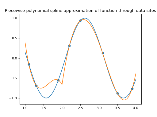
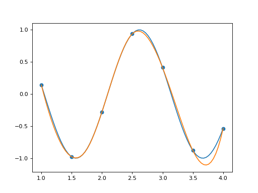
In this case, omitting the continuity conditions at the interior breakpoint, 2, creates quite a problem. For the purpose of using this module within the Curve class we always use full continuity at the interior breakpoints. 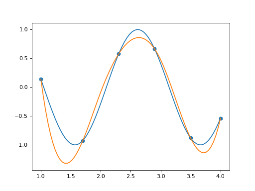If we remove two dimensions of the spline (to yield dimension 6) by imposing further continuity of derivative and second derivative at $\xi=2$ (and 2 data sites to match the new spline dimension and yield a square linear system), then we obtain a more reasonable spline approximation of this function.

In [15]: spline = PPSplineF64(k=4, t=[1,1,1,1,2,3,4,4,4,4])

In [16]: tau = np.array([1.0, 1.7, 2.3, 2.9, 3.5, 4.0])

In [17]: spline.csolve(tau, np.sin(3*tau), 0, 0, False)

In [18]: fig, ax = plt.subplots(1,1)

In [19]: ax.plot(x, np.sin(3*x))
Out[19]: [<matplotlib.lines.Line2D at 0x7f0aa034d210>]

In [20]: ax.scatter(tau, np.sin(3*tau))
Out[20]: <matplotlib.collections.PathCollection at 0x7f0aa033ba90>

In [21]: ax.plot(x, spline.ppev(x))
Out[21]: [<matplotlib.lines.Line2D at 0x7f0aa179f990>]

(Source code, png, hires.png, pdf)

The accuracy of the approximation in this case can be improved either by:

utilising better placed data sites,
increasing the dimension of the spline (and the associated degrees of freedom) by inserting further interior breakpoints and increasing the number of data sites,
keeping the dimension of the spline and increasing the number of data sites and allowing those data sites to solve with error minimised under least squares.

The below demonstrates increasing the spline dimension to 7 and adding a data site.

In [22]: spline = PPSplineF64(k=4, t=[1,1,1,1,1.75,2.5,3.25,4,4,4,4])

In [23]: tau = np.array([1.0, 1.5, 2.0, 2.5, 3, 3.5, 4.0])

In [24]: spline.csolve(tau, np.sin(3*tau), 0, 0, False)

In [25]: fig, ax = plt.subplots(1,1)

In [26]: ax.plot(x, np.sin(3*x))
Out[26]: [<matplotlib.lines.Line2D at 0x7f0aa11e2290>]

In [27]: ax.scatter(tau, np.sin(3*tau))
Out[27]: <matplotlib.collections.PathCollection at 0x7f0aa02c5210>

In [28]: ax.plot(x, spline.ppev(x))
Out[28]: [<matplotlib.lines.Line2D at 0x7f0aa00ffb10>]

(Source code, png, hires.png, pdf)

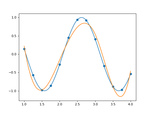
Alternatively we demonstrate keeping the original spline dimension of 6 and adding more data sites and solving with least squares error. In this case the accuracy of the spline is somewhat constrained by its limiting degrees of freedom.

In [29]: spline = PPSplineF64(k=4, t=[1,1,1,1,2,3,4,4,4,4])

In [30]: tau = np.array([1.0, 1.25, 1.5, 1.75, 2.0, 2.25, 2.5, 2.75, 3, 3.25, 3.5, 3.75, 4.0])

In [31]: spline.csolve(tau, np.sin(3*tau), 0, 0, allow_lsq=True)

In [32]: fig, ax = plt.subplots(1,1)

In [33]: ax.plot(x, np.sin(3*x))
Out[33]: [<matplotlib.lines.Line2D at 0x7f0aa032c810>]

In [34]: ax.scatter(tau, np.sin(3*tau))
Out[34]: <matplotlib.collections.PathCollection at 0x7f0aa1095b10>

In [35]: ax.plot(x, spline.ppev(x))
Out[35]: [<matplotlib.lines.Line2D at 0x7f0aa129f210>]

(Source code, png, hires.png, pdf)

Endpoint Constraints#

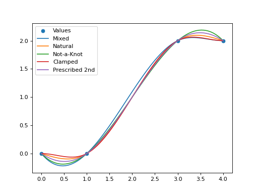
The various end point constraints can be generated in this implementation:

Natural spline: this enforces second order derivative equal to zero at the endpoints. This is most useful for splines of order 4 (cubic) and higher.
Prescribed second derivative: this enforces second order derivative of given values at the endpoints. Also useful for order 4 and higher.
Clamped spline: this enforces first order derivative of a given value at the endpoints. This is useful for order 3 and higher.
Not-a-knot: this enforces third order derivative continuity at the 2nd and penultimate breakpoints. This is most often used with order 4 splines.
Function value: this enforces the spline to take specific values at the endpoints and the rest of the spline is determined by data site and function values. This can be used with any order spline.
Mixed constraints: this allows combinations of the above methods at each end.

Suppose we wish to generate between the points (0,0), (1,0), (3,2), (4,2), as demonstrated in this spline note published by the school of computer science at Tel Aviv University, then we can generate the following splines using this library in the following way:

Natural Spline#

In [36]: t = [0, 0, 0, 0, 1, 3, 4, 4, 4, 4]

In [37]: spline = PPSplineF64(k=4, t=t)

In [38]: tau = np.array([0, 0, 1, 3, 4, 4])

In [39]: val = np.array([0, 0, 0, 2, 2, 0])

In [40]: spline.csolve(tau, val, 2, 2, False)

Second derivative values of zero have been added to the data sites, $\tau$. The csolve() function is set to use second derivatives.

Prescribed Second Derivatives#

In [41]: t = [0, 0, 0, 0, 1, 3, 4, 4, 4, 4]

In [42]: spline = PPSplineF64(k=4, t=t)

In [43]: tau = np.array([0, 0, 1, 3, 4, 4])

In [44]: val = np.array([1, 0, 0, 2, 2, -1])

In [45]: spline.csolve(tau, val, 2, 2, False)

Here, second derivative values of specific values 1 and -1 have been set.

Clamped Spline#

In [46]: t = [0, 0, 0, 0, 1, 3, 4, 4, 4, 4]

In [47]: spline = PPSplineF64(k=4, t=t)

In [48]: tau = np.array([0, 0, 1, 3, 4, 4])

In [49]: val = np.array([0, 0, 0, 2, 2, 0])

In [50]: spline.csolve(tau, val, 1, 1, False)

In this case first derivative values of zero have been set and the csolve() function updated.

Not-a-Knot Spline#

In [51]: t = [0, 0, 0, 0, 4, 4, 4, 4]

In [52]: spline = PPSplineF64(k=4, t=t)

In [53]: tau = np.array([0, 1, 3, 4])

In [54]: val = np.array([0, 0, 2, 2])

In [55]: spline.csolve(tau, val, 0, 0, False)

Note that the removal of the interior breakpoints (as implied by the name) has been required here in the knot sequence, t.

The not-a-knot spline also demonstrate the pure function value spline since csolve() uses function values at the endpoints.

Mixed Spline#

In [56]: t = [0, 0, 0, 0, 3, 4, 4, 4, 4]

In [57]: spline = PPSplineF64(k=4, t=t)

In [58]: tau = np.array([0, 1, 3, 4, 4])

In [59]: val = np.array([0, 0, 2, 2, 0])

In [60]: spline.csolve(tau, val, 0, 1, False)

Mixed splines can be generated by combining, e.g. the above combines not-a-knot left side with a clamped right side.

(Source code, png, hires.png, pdf)

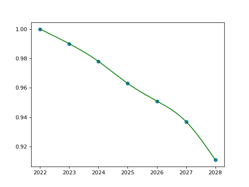
Application to Discount Factors#

The specific use case for this module in this library is for log-cubic splines over discount factors. Suppose we have the following node dates and discount factors at those points:

2022-1-1: 1.000
2023-1-1: 0.990
2024-1-1: 0.978
2025-1-1: 0.963
2026-1-1: 0.951
2027-1-1: 0.937
2028-1-1: 0.911

We seek a spline interpolator for these points. The basic concept is to construct a PPSplineF64 and then solve for the b-spline coefficients using the logarithm of the discount factors at the given dates. In fact, we add two conditions for a natural spline which is to suggest that curvature at the endpoint is minimised to zero, i.e. we set the second derivative of the spline to zero at the endpoints. This is added specifically to our data sites and to our spline collocation matrix. The internal workings of the Curve class perform exactly the steps as outlined in the below manual example.

In [61]: from pytz import UTC

In [62]: tau = [dt(2022,1,1), dt(2023,1,1), dt(2024,1,1), dt(2025,1,1), dt(2026,1,1), dt(2027,1,1), dt(2028,1,1)]

In [63]: tau_posix = [_.replace(tzinfo=UTC).timestamp() for _ in tau]

In [64]: df = np.array([1.0, 0.99, 0.978, 0.963, 0.951, 0.937, 0.911])

In [65]: y = np.log(df)

In [66]: t = [dt(2022,1,1), dt(2022,1,1), dt(2022,1,1), dt(2022,1,1), dt(2023,1,1), dt(2024,1,1), dt(2025,1,1), dt(2026,1,1), dt(2027,1,1), dt(2028,1,1), dt(2028,1,1), dt(2028,1,1), dt(2028,1,1)]

In [67]: t_posix = [_.replace(tzinfo=UTC).timestamp() for _ in t]

In [68]: spline = PPSplineF64(k=4, t=t_posix)

# we create a natural spline by setting the second derivative at endpoints to zero
# so we artificially add two endpoint data sites
In [69]: tau_augmented = tau_posix.copy()

In [70]: tau_augmented.insert(0, dt(2022,1,1).replace(tzinfo=UTC).timestamp())

In [71]: tau_augmented.append(dt(2028,1,1).replace(tzinfo=UTC).timestamp())

In [72]: y_augmented = np.zeros(len(y)+2)

In [73]: y_augmented[1:-1] = y

In [74]: spline.csolve(tau_augmented, y_augmented, 2, 2, False)

In [75]: fig, ax = plt.subplots(1,1)

In [76]: ax.scatter(tau, df)
Out[76]: <matplotlib.collections.PathCollection at 0x7f0aa0a22110>

In [77]: x = [dt(2022,1,1) + timedelta(days=2*i) for i in range(365*3)]

In [78]: x_posix = [_.replace(tzinfo=UTC).timestamp() for _ in x]

In [79]: ax.plot(x, np.exp(spline.ppev(np.array(x_posix))), color="g")
Out[79]: [<matplotlib.lines.Line2D at 0x7f0aa0c04a90>]

(Source code, png, hires.png, pdf)

AD and Working with Dual and Dual2#

Splines in rateslib are designed to be fully integrated into the forward mode AD used within the library. This means that both:

Sensitivities to the y-axis datapoints can be captured.
Sensitivities to the x-axis indexing can also be captured.

Sensitivities to y-axis datapoints#

To capture A) 3 splines are available for the specific calculation mode: PPSplineF64, PPSplineDual and PPSplineDual2. Choose to use the appropriate Dual version depending upon which derivatives you wish to capture.

For example, suppose we rebuild the natural spline from the endpoints section above. But this time the 4 data points are labelled as variables referencing the y-axis:

In [80]: pps = PPSplineDual(t=[0, 0, 0, 0, 1, 3, 4, 4, 4, 4], k=4)

In [81]: pps.csolve(
   ....:     tau=[0, 0, 1, 3, 4, 4],
   ....:     y=[
   ....:         Dual(0, [], []),
   ....:         Dual(0, ["y0"], []),
   ....:         Dual(0, ["y1"], []),
   ....:         Dual(2, ["y2"], []),
   ....:         Dual(2, ["y3"], []),
   ....:         Dual(0, [], [])
   ....:     ],
   ....:     left_n=2,
   ....:     right_n=2,
   ....:     allow_lsq=False,
   ....: )
   ....: 

Now, when we interrogate the spline for a given x-value, say 3.5, the returned value will demonstrate the sensitivity of that value to the movement in any of the values y0, y1, y2, or y3.

In [82]: pps.ppev_single(3.5)
Out[82]: <Dual: 2.093750, (y3, y0, y1, ...), [0.4, 0.0, -0.1, ...]>

This suggests that if y3 were to move up by an infinitesimal amount, say 0.0001, then the y-value associated with an x-value of 3.5 would be 0.00004 higher or rather 2.09379.

In [83]: pps_f64 = PPSplineF64(t=[0, 0, 0, 0, 1, 3, 4, 4, 4, 4], k=4)

In [84]: pps_f64.csolve(
   ....:     tau=[0, 0, 1, 3, 4, 4],
   ....:     y=[0, 0, 0, 2, 2.0001, 0],
   ....:     left_n=2,
   ....:     right_n=2,
   ....:     allow_lsq=False,
   ....: )
   ....: 

In [85]: pps_f64.ppev_single(3.5)
Out[85]: 2.09379296875

Sensitivities to x-axis datapoints#

To demonstrate B), suppose we wish to capture the sensitivity of that y-value as the x-value were to vary. We can do this in two ways. The first is to use the analytical function for the derivative of a spline:

In [86]: pps_f64.ppdnev_single(3.5, 1)
Out[86]: -0.06239531249999897

The second is to interrogate the spline with the x-value set as a variable.

In [87]: pps_f64.ppev_single_dual(Dual(3.5, ["x"], [])).dual
Out[87]: array([-0.06239531])

Three functions exist for extracting spline values for each case: ppev_single(), ppev_single_dual(), ppev_single_dual2(),

Rateslib recommends the use of the evaluate() method, however, since this method will automatically choose the appropriate method above to call and return the value with the correct AD sensitivity.

	y-values
x-values	Float	Dual	Dual2
Float	PPSplineF64, and ppev_single()	PPSplineDual, and ppev_single()	PPSplineDual2, and ppev_single()
Dual	PPSplineF64, and ppev_single_dual()	PPSplineDual, and ppev_single_dual()	TypeError
Dual2	PPSplineF64, and ppev_single_dual2()	TypeError	PPSplineDual2, and ppev_single_dual2()

Simultaneous sensitivities to extraneous variables#

The following example is more general and demonstrates the power of having spline interpolator functions whose derivatives are fully integrated into the toolset. This is one of the advantages of adopting forward mode derivatives with dual numbers.

Suppose now that everything is sensitive to an extraneous variable, say z. The sensitivies of each element to z are constructed as below:

In [88]: y0 = Dual(0, ["z"], [2.0])

In [89]: y1 = Dual(0, ["z"], [-3.0])

In [90]: y2 = Dual(2, ["z"], [4.0])

In [91]: y3 = Dual(2, ["z"], [10.0])

In [92]: x = Dual(3.5, ["z"], [-5.0])

We construct a spline and measure the resulting interpolated y-value’s sensitivity to z.

In [93]: pps = PPSplineDual(t=[0, 0, 0, 0, 1, 3, 4, 4, 4, 4], k=4)

In [94]: pps.csolve(
   ....:     tau=[0, 0, 1, 3, 4, 4],
   ....:     y=[Dual(0, [], []), y0, y1, y2, y3, Dual(0, [], [])],
   ....:     left_n=2,
   ....:     right_n=2,
   ....:     allow_lsq=False,
   ....: )
   ....: 

In [95]: evaluate(pps, x)
Out[95]: <Dual: 2.093750, (z), [7.3]>

This suggests that if z moves 0.0001 higher then this value should move by 0.00073 higher to 2.09448. But of course all of the all x and y values have sensitivity to z as well.

In [96]: pps = PPSplineF64(t=[0, 0, 0, 0, 1, 3, 4, 4, 4, 4], k=4)

In [97]: pps.csolve(
   ....:     tau=[0, 0, 1, 3, 4, 4],
   ....:     y=[0, 0.0002, -0.0003, 2.0004, 2.001, 0],
   ....:     left_n=2,
   ....:     right_n=2,
   ....:     allow_lsq=False,
   ....: )
   ....: 

In [98]: evaluate(pps, 3.4995)
Out[98]: 2.094483200747655

As predicted!